descriptive research based on data

• Skip to main content
• Skip to primary sidebar
• Skip to footer
• QuestionPro

• Solutions Industries Gaming Automotive Sports and events Education Government Travel & Hospitality Financial Services Healthcare Cannabis Technology Use Case AskWhy Communities Audience Contactless surveys Mobile LivePolls Member Experience GDPR Positive People Science 360 Feedback Surveys
• Resources Blog eBooks Survey Templates Case Studies Training Help center

Home Market Research

Descriptive Research: Definition, Characteristics, Methods + Examples

Suppose an apparel brand wants to understand the fashion purchasing trends among New York’s buyers, then it must conduct a demographic survey of the specific region, gather population data, and then conduct descriptive research on this demographic segment.

The study will then uncover details on “what is the purchasing pattern of New York buyers,” but will not cover any investigative information about “ why ” the patterns exist. Because for the apparel brand trying to break into this market, understanding the nature of their market is the study’s main goal. Let’s talk about it.

What is descriptive research?

Descriptive research is a research method describing the characteristics of the population or phenomenon studied. This descriptive methodology focuses more on the “what” of the research subject than the “why” of the research subject.

The method primarily focuses on describing the nature of a demographic segment without focusing on “why” a particular phenomenon occurs. In other words, it “describes” the research subject without covering “why” it happens.

Characteristics of descriptive research

The term descriptive research then refers to research questions, the design of the study, and data analysis conducted on that topic. We call it an observational research method because none of the research study variables are influenced in any capacity.

Some distinctive characteristics of descriptive research are:

• Quantitative research: It is a quantitative research method that attempts to collect quantifiable information for statistical analysis of the population sample. It is a popular market research tool that allows us to collect and describe the demographic segment’s nature.
• Uncontrolled variables: In it, none of the variables are influenced in any way. This uses observational methods to conduct the research. Hence, the nature of the variables or their behavior is not in the hands of the researcher.
• Cross-sectional studies: It is generally a cross-sectional study where different sections belonging to the same group are studied.
• The basis for further research: Researchers further research the data collected and analyzed from descriptive research using different research techniques. The data can also help point towards the types of research methods used for the subsequent research.

Applications of descriptive research with examples

A descriptive research method can be used in multiple ways and for various reasons. Before getting into any survey , though, the survey goals and survey design are crucial. Despite following these steps, there is no way to know if one will meet the research outcome. How to use descriptive research? To understand the end objective of research goals, below are some ways organizations currently use descriptive research today:

• Define respondent characteristics: The aim of using close-ended questions is to draw concrete conclusions about the respondents. This could be the need to derive patterns, traits, and behaviors of the respondents. It could also be to understand from a respondent their attitude, or opinion about the phenomenon. For example, understand millennials and the hours per week they spend browsing the internet. All this information helps the organization researching to make informed business decisions.
• Measure data trends: Researchers measure data trends over time with a descriptive research design’s statistical capabilities. Consider if an apparel company researches different demographics like age groups from 24-35 and 36-45 on a new range launch of autumn wear. If one of those groups doesn’t take too well to the new launch, it provides insight into what clothes are like and what is not. The brand drops the clothes and apparel that customers don’t like.
• Conduct comparisons: Organizations also use a descriptive research design to understand how different groups respond to a specific product or service. For example, an apparel brand creates a survey asking general questions that measure the brand’s image. The same study also asks demographic questions like age, income, gender, geographical location, geographic segmentation , etc. This consumer research helps the organization understand what aspects of the brand appeal to the population and what aspects do not. It also helps make product or marketing fixes or even create a new product line to cater to high-growth potential groups.
• Validate existing conditions: Researchers widely use descriptive research to help ascertain the research object’s prevailing conditions and underlying patterns. Due to the non-invasive research method and the use of quantitative observation and some aspects of qualitative observation , researchers observe each variable and conduct an in-depth analysis . Researchers also use it to validate any existing conditions that may be prevalent in a population.
• Conduct research at different times: The analysis can be conducted at different periods to ascertain any similarities or differences. This also allows any number of variables to be evaluated. For verification, studies on prevailing conditions can also be repeated to draw trends.

Advantages of descriptive research

Some of the significant advantages of descriptive research are:

• Data collection: A researcher can conduct descriptive research using specific methods like observational method, case study method, and survey method. Between these three, all primary data collection methods are covered, which provides a lot of information. This can be used for future research or even for developing a hypothesis for your research object.
• Varied: Since the data collected is qualitative and quantitative, it gives a holistic understanding of a research topic. The information is varied, diverse, and thorough.
• Natural environment: Descriptive research allows for the research to be conducted in the respondent’s natural environment, which ensures that high-quality and honest data is collected.
• Quick to perform and cheap: As the sample size is generally large in descriptive research, the data collection is quick to conduct and is inexpensive.

Descriptive research methods

There are three distinctive methods to conduct descriptive research. They are:

Observational method

The observational method is the most effective method to conduct this research, and researchers make use of both quantitative and qualitative observations.

A quantitative observation is the objective collection of data primarily focused on numbers and values. It suggests “associated with, of or depicted in terms of a quantity.” Results of quantitative observation are derived using statistical and numerical analysis methods. It implies observation of any entity associated with a numeric value such as age, shape, weight, volume, scale, etc. For example, the researcher can track if current customers will refer the brand using a simple Net Promoter Score question .

Qualitative observation doesn’t involve measurements or numbers but instead just monitoring characteristics. In this case, the researcher observes the respondents from a distance. Since the respondents are in a comfortable environment, the characteristics observed are natural and effective. In a descriptive research design, the researcher can choose to be either a complete observer, an observer as a participant, a participant as an observer, or a full participant. For example, in a supermarket, a researcher can from afar monitor and track the customers’ selection and purchasing trends. This offers a more in-depth insight into the purchasing experience of the customer.

Case study method

Case studies involve in-depth research and study of individuals or groups. Case studies lead to a hypothesis and widen a further scope of studying a phenomenon. However, case studies should not be used to determine cause and effect as they can’t make accurate predictions because there could be a bias on the researcher’s part. The other reason why case studies are not a reliable way of conducting descriptive research is that there could be an atypical respondent in the survey. Describing them leads to weak generalizations and moving away from external validity.

Survey research

In survey research, respondents answer through surveys or questionnaires or polls . They are a popular market research tool to collect feedback from respondents. A study to gather useful data should have the right survey questions. It should be a balanced mix of open-ended questions and close ended-questions . The survey method can be conducted online or offline, making it the go-to option for descriptive research where the sample size is enormous.

Examples of descriptive research

Some examples of descriptive research are:

• A specialty food group launching a new range of barbecue rubs would like to understand what flavors of rubs are favored by different people. To understand the preferred flavor palette, they conduct this type of research study using various methods like observational methods in supermarkets. By also surveying while collecting in-depth demographic information, offers insights about the preference of different markets. This can also help tailor make the rubs and spreads to various preferred meats in that demographic. Conducting this type of research helps the organization tweak their business model and amplify marketing in core markets.
• Another example of where this research can be used is if a school district wishes to evaluate teachers’ attitudes about using technology in the classroom. By conducting surveys and observing their comfortableness using technology through observational methods, the researcher can gauge what they can help understand if a full-fledged implementation can face an issue. This also helps in understanding if the students are impacted in any way with this change.

Some other research problems and research questions that can lead to descriptive research are:

• Market researchers want to observe the habits of consumers.
• A company wants to evaluate the morale of its staff.
• A school district wants to understand if students will access online lessons rather than textbooks.
• To understand if its wellness questionnaire programs enhance the overall health of the employees.

LEARN MORE         FREE TRIAL

MORE LIKE THIS

Was The Experience Memorable? — Tuesday CX Thoughts

Sep 10, 2024

What Does a Data Analyst Do? Skills, Tools & Tips

Sep 9, 2024

Best Gallup Access Alternatives & Competitors in 2024

Sep 6, 2024

Experimental vs Observational Studies: Differences & Examples

Sep 5, 2024

Other categories

• Academic Research
• Artificial Intelligence
• Assessments
• Brand Awareness
• Case Studies
• Communities
• Consumer Insights
• Customer effort score
• Customer Engagement
• Customer Experience
• Customer Loyalty
• Customer Research
• Customer Satisfaction
• Employee Benefits
• Employee Engagement
• Employee Retention
• Friday Five
• General Data Protection Regulation
• Insights Hub
• Life@QuestionPro
• Market Research
• Mobile diaries
• Mobile Surveys
• New Features
• Online Communities
• Question Types
• Questionnaire
• QuestionPro Products
• Release Notes
• Research Tools and Apps
• Revenue at Risk
• Survey Templates
• Training Tips
• Tuesday CX Thoughts (TCXT)
• Uncategorized
• What’s Coming Up
• Workforce Intelligence

• Descriptive Research Designs: Types, Examples & Methods

One of the components of research is getting enough information about the research problem—the what, how, when and where answers, which is why descriptive research is an important type of research. It is very useful when conducting research whose aim is to identify characteristics, frequencies, trends, correlations, and categories.

This research method takes a problem with little to no relevant information and gives it a befitting description using qualitative and quantitative research method s. Descriptive research aims to accurately describe a research problem.

In the subsequent sections, we will be explaining what descriptive research means, its types, examples, and data collection methods.

What is Descriptive Research?

Descriptive research is a type of research that describes a population, situation, or phenomenon that is being studied. It focuses on answering the how, what, when, and where questions If a research problem, rather than the why.

This is mainly because it is important to have a proper understanding of what a research problem is about before investigating why it exists in the first place. 

For example, an investor considering an investment in the ever-changing Amsterdam housing market needs to understand what the current state of the market is, how it changes (increasing or decreasing), and when it changes (time of the year) before asking for the why. This is where descriptive research comes in.

What Are The Types of Descriptive Research?

Descriptive research is classified into different types according to the kind of approach that is used in conducting descriptive research. The different types of descriptive research are highlighted below:

• Descriptive-survey

Descriptive survey research uses surveys to gather data about varying subjects. This data aims to know the extent to which different conditions can be obtained among these subjects.

For example, a researcher wants to determine the qualification of employed professionals in Maryland. He uses a survey as his research instrument , and each item on the survey related to qualifications is subjected to a Yes/No answer. 

This way, the researcher can describe the qualifications possessed by the employed demographics of this community. 

• Descriptive-normative survey

This is an extension of the descriptive survey, with the addition being the normative element. In the descriptive-normative survey, the results of the study should be compared with the norm.

For example, an organization that wishes to test the skills of its employees by a team may have them take a skills test. The skills tests are the evaluation tool in this case, and the result of this test is compared with the norm of each role.

If the score of the team is one standard deviation above the mean, it is very satisfactory, if within the mean, satisfactory, and one standard deviation below the mean is unsatisfactory.

• Descriptive-status

This is a quantitative description technique that seeks to answer questions about real-life situations. For example, a researcher researching the income of the employees in a company, and the relationship with their performance.

A survey will be carried out to gather enough data about the income of the employees, then their performance will be evaluated and compared to their income. This will help determine whether a higher income means better performance and low income means lower performance or vice versa.

• Descriptive-analysis

The descriptive-analysis method of research describes a subject by further analyzing it, which in this case involves dividing it into 2 parts. For example, the HR personnel of a company that wishes to analyze the job role of each employee of the company may divide the employees into the people that work at the Headquarters in the US and those that work from Oslo, Norway office.

A questionnaire is devised to analyze the job role of employees with similar salaries and who work in similar positions.

• Descriptive classification

This method is employed in biological sciences for the classification of plants and animals. A researcher who wishes to classify the sea animals into different species will collect samples from various search stations, then classify them accordingly.

• Descriptive-comparative

In descriptive-comparative research, the researcher considers 2 variables that are not manipulated, and establish a formal procedure to conclude that one is better than the other. For example, an examination body wants to determine the better method of conducting tests between paper-based and computer-based tests.

A random sample of potential participants of the test may be asked to use the 2 different methods, and factors like failure rates, time factors, and others will be evaluated to arrive at the best method.

• Correlative Survey

Correlative surveys are used to determine whether the relationship between 2 variables is positive, negative, or neutral. That is, if 2 variables say X and Y are directly proportional, inversely proportional or are not related to each other.

Examples of Descriptive Research

There are different examples of descriptive research, that may be highlighted from its types, uses, and applications. However, we will be restricting ourselves to only 3 distinct examples in this article.

• Comparing Student Performance:

An academic institution may wish 2 compare the performance of its junior high school students in English language and Mathematics. This may be used to classify students based on 2 major groups, with one group going ahead to study while courses, while the other study courses in the Arts & Humanities field.

Students who are more proficient in mathematics will be encouraged to go into STEM and vice versa. Institutions may also use this data to identify students’ weak points and work on ways to assist them.

• Scientific Classification

During the major scientific classification of plants, animals, and periodic table elements, the characteristics and components of each subject are evaluated and used to determine how they are classified.

For example, living things may be classified into kingdom Plantae or kingdom animal is depending on their nature. Further classification may group animals into mammals, pieces, vertebrae, invertebrae, etc. 

All these classifications are made a result of descriptive research which describes what they are.

• Human Behavior

When studying human behaviour based on a factor or event, the researcher observes the characteristics, behaviour, and reaction, then use it to conclude. A company willing to sell to its target market needs to first study the behaviour of the market.

This may be done by observing how its target reacts to a competitor’s product, then use it to determine their behaviour.

What are the Characteristics of Descriptive Research?  

The characteristics of descriptive research can be highlighted from its definition, applications, data collection methods, and examples. Some characteristics of descriptive research are:

• Quantitativeness

Descriptive research uses a quantitative research method by collecting quantifiable information to be used for statistical analysis of the population sample. This is very common when dealing with research in the physical sciences.

• Qualitativeness

It can also be carried out using the qualitative research method, to properly describe the research problem. This is because descriptive research is more explanatory than exploratory or experimental.

• Uncontrolled variables

In descriptive research, researchers cannot control the variables like they do in experimental research.

• The basis for further research

The results of descriptive research can be further analyzed and used in other research methods. It can also inform the next line of research, including the research method that should be used.

This is because it provides basic information about the research problem, which may give birth to other questions like why a particular thing is the way it is.

Why Use Descriptive Research Design?  

Descriptive research can be used to investigate the background of a research problem and get the required information needed to carry out further research. It is used in multiple ways by different organizations, and especially when getting the required information about their target audience.

• Define subject characteristics :

It is used to determine the characteristics of the subjects, including their traits, behaviour, opinion, etc. This information may be gathered with the use of surveys, which are shared with the respondents who in this case, are the research subjects.

For example, a survey evaluating the number of hours millennials in a community spends on the internet weekly, will help a service provider make informed business decisions regarding the market potential of the community.

• Measure Data Trends

It helps to measure the changes in data over some time through statistical methods. Consider the case of individuals who want to invest in stock markets, so they evaluate the changes in prices of the available stocks to make a decision investment decision.

Brokerage companies are however the ones who carry out the descriptive research process, while individuals can view the data trends and make decisions.

Descriptive research is also used to compare how different demographics respond to certain variables. For example, an organization may study how people with different income levels react to the launch of a new Apple phone.

This kind of research may take a survey that will help determine which group of individuals are purchasing the new Apple phone. Do the low-income earners also purchase the phone, or only the high-income earners do?

Further research using another technique will explain why low-income earners are purchasing the phone even though they can barely afford it. This will help inform strategies that will lure other low-income earners and increase company sales.

• Validate existing conditions

When you are not sure about the validity of an existing condition, you can use descriptive research to ascertain the underlying patterns of the research object. This is because descriptive research methods make an in-depth analysis of each variable before making conclusions.

• Conducted Overtime

Descriptive research is conducted over some time to ascertain the changes observed at each point in time. The higher the number of times it is conducted, the more authentic the conclusion will be.

What are the Disadvantages of Descriptive Research?  

• Response and Non-response Bias

Respondents may either decide not to respond to questions or give incorrect responses if they feel the questions are too confidential. When researchers use observational methods, respondents may also decide to behave in a particular manner because they feel they are being watched.

• The researcher may decide to influence the result of the research due to personal opinion or bias towards a particular subject. For example, a stockbroker who also has a business of his own may try to lure investors into investing in his own company by manipulating results.
• A case-study or sample taken from a large population is not representative of the whole population.
• Limited scope:The scope of descriptive research is limited to the what of research, with no information on why thereby limiting the scope of the research.

What are the Data Collection Methods in Descriptive Research?  

There are 3 main data collection methods in descriptive research, namely; observational method, case study method, and survey research.

1. Observational Method

The observational method allows researchers to collect data based on their view of the behaviour and characteristics of the respondent, with the respondents themselves not directly having an input. It is often used in market research, psychology, and some other social science research to understand human behaviour.

It is also an important aspect of physical scientific research, with it being one of the most effective methods of conducting descriptive research . This process can be said to be either quantitative or qualitative.

Quantitative observation involved the objective collection of numerical data , whose results can be analyzed using numerical and statistical methods. 

Qualitative observation, on the other hand, involves the monitoring of characteristics and not the measurement of numbers. The researcher makes his observation from a distance, records it, and is used to inform conclusions.

2. Case Study Method

A case study is a sample group (an individual, a group of people, organizations, events, etc.) whose characteristics are used to describe the characteristics of a larger group in which the case study is a subgroup. The information gathered from investigating a case study may be generalized to serve the larger group.

This generalization, may, however, be risky because case studies are not sufficient to make accurate predictions about larger groups. Case studies are a poor case of generalization.

3. Survey Research

This is a very popular data collection method in research designs. In survey research, researchers create a survey or questionnaire and distribute it to respondents who give answers.

Generally, it is used to obtain quick information directly from the primary source and also conducting rigorous quantitative and qualitative research. In some cases, survey research uses a blend of both qualitative and quantitative strategies.

Survey research can be carried out both online and offline using the following methods

• Online Surveys: This is a cheap method of carrying out surveys and getting enough responses. It can be carried out using Formplus, an online survey builder. Formplus has amazing tools and features that will help increase response rates.
• Offline Surveys: This includes paper forms, mobile offline forms , and SMS-based forms.

What Are The Differences Between Descriptive and Correlational Research?  

Before going into the differences between descriptive and correlation research, we need to have a proper understanding of what correlation research is about. Therefore, we will be giving a summary of the correlation research below.

Correlational research is a type of descriptive research, which is used to measure the relationship between 2 variables, with the researcher having no control over them. It aims to find whether there is; positive correlation (both variables change in the same direction), negative correlation (the variables change in the opposite direction), or zero correlation (there is no relationship between the variables).

Correlational research may be used in 2 situations;

(i) when trying to find out if there is a relationship between two variables, and

(ii) when a causal relationship is suspected between two variables, but it is impractical or unethical to conduct experimental research that manipulates one of the variables. 

Below are some of the differences between correlational and descriptive research:

• Definitions :

Descriptive research aims is a type of research that provides an in-depth understanding of the study population, while correlational research is the type of research that measures the relationship between 2 variables. 

• Characteristics :

Descriptive research provides descriptive data explaining what the research subject is about, while correlation research explores the relationship between data and not their description.

• Predictions :

 Predictions cannot be made in descriptive research while correlation research accommodates the possibility of making predictions.

Descriptive Research vs. Causal Research

Descriptive research and causal research are both research methodologies, however, one focuses on a subject’s behaviors while the latter focuses on a relationship’s cause-and-effect. To buttress the above point, descriptive research aims to describe and document the characteristics, behaviors, or phenomena of a particular or specific population or situation. 

It focuses on providing an accurate and detailed account of an already existing state of affairs between variables. Descriptive research answers the questions of “what,” “where,” “when,” and “how” without attempting to establish any causal relationships or explain any underlying factors that might have caused the behavior.

Causal research, on the other hand, seeks to determine cause-and-effect relationships between variables. It aims to point out the factors that influence or cause a particular result or behavior. Causal research involves manipulating variables, controlling conditions or a subgroup, and observing the resulting effects. The primary objective of causal research is to establish a cause-effect relationship and provide insights into why certain phenomena happen the way they do.

Descriptive Research vs. Analytical Research

Descriptive research provides a detailed and comprehensive account of a specific situation or phenomenon. It focuses on describing and summarizing data without making inferences or attempting to explain underlying factors or the cause of the factor. 

It is primarily concerned with providing an accurate and objective representation of the subject of research. While analytical research goes beyond the description of the phenomena and seeks to analyze and interpret data to discover if there are patterns, relationships, or any underlying factors. 

It examines the data critically, applies statistical techniques or other analytical methods, and draws conclusions based on the discovery. Analytical research also aims to explore the relationships between variables and understand the underlying mechanisms or processes involved.

Descriptive Research vs. Exploratory Research

Descriptive research is a research method that focuses on providing a detailed and accurate account of a specific situation, group, or phenomenon. This type of research describes the characteristics, behaviors, or relationships within the given context without looking for an underlying cause. 

Descriptive research typically involves collecting and analyzing quantitative or qualitative data to generate descriptive statistics or narratives. Exploratory research differs from descriptive research because it aims to explore and gain firsthand insights or knowledge into a relatively unexplored or poorly understood topic. 

It focuses on generating ideas, hypotheses, or theories rather than providing definitive answers. Exploratory research is often conducted at the early stages of a research project to gather preliminary information and identify key variables or factors for further investigation. It involves open-ended interviews, observations, or small-scale surveys to gather qualitative data.

Read More – Exploratory Research: What are its Method & Examples?

Descriptive Research vs. Experimental Research

Descriptive research aims to describe and document the characteristics, behaviors, or phenomena of a particular population or situation. It focuses on providing an accurate and detailed account of the existing state of affairs. 

Descriptive research typically involves collecting data through surveys, observations, or existing records and analyzing the data to generate descriptive statistics or narratives. It does not involve manipulating variables or establishing cause-and-effect relationships.

Experimental research, on the other hand, involves manipulating variables and controlling conditions to investigate cause-and-effect relationships. It aims to establish causal relationships by introducing an intervention or treatment and observing the resulting effects. 

Experimental research typically involves randomly assigning participants to different groups, such as control and experimental groups, and measuring the outcomes. It allows researchers to control for confounding variables and draw causal conclusions.

Related – Experimental vs Non-Experimental Research: 15 Key Differences

Descriptive Research vs. Explanatory Research

Descriptive research focuses on providing a detailed and accurate account of a specific situation, group, or phenomenon. It aims to describe the characteristics, behaviors, or relationships within the given context. 

Descriptive research is primarily concerned with providing an objective representation of the subject of study without explaining underlying causes or mechanisms. Explanatory research seeks to explain the relationships between variables and uncover the underlying causes or mechanisms. 

It goes beyond description and aims to understand the reasons or factors that influence a particular outcome or behavior. Explanatory research involves analyzing data, conducting statistical analyses, and developing theories or models to explain the observed relationships.

Descriptive Research vs. Inferential Research

Descriptive research focuses on describing and summarizing data without making inferences or generalizations beyond the specific sample or population being studied. It aims to provide an accurate and objective representation of the subject of study. 

Descriptive research typically involves analyzing data to generate descriptive statistics, such as means, frequencies, or percentages, to describe the characteristics or behaviors observed.

Inferential research, however, involves making inferences or generalizations about a larger population based on a smaller sample. 

It aims to draw conclusions about the population characteristics or relationships by analyzing the sample data. Inferential research uses statistical techniques to estimate population parameters, test hypotheses, and determine the level of confidence or significance in the findings.

Related – Inferential Statistics: Definition, Types + Examples

Conclusion  

The uniqueness of descriptive research partly lies in its ability to explore both quantitative and qualitative research methods. Therefore, when conducting descriptive research, researchers have the opportunity to use a wide variety of techniques that aids the research process.

Descriptive research explores research problems in-depth, beyond the surface level thereby giving a detailed description of the research subject. That way, it can aid further research in the field, including other research methods .

It is also very useful in solving real-life problems in various fields of social science, physical science, and education.

Connect to Formplus, Get Started Now - It's Free!

• descriptive research
• descriptive research method
• example of descriptive research
• types of descriptive research
• busayo.longe

You may also like:

Extrapolation in Statistical Research: Definition, Examples, Types, Applications

In this article we’ll look at the different types and characteristics of extrapolation, plus how it contrasts to interpolation.

Cross-Sectional Studies: Types, Pros, Cons & Uses

In this article, we’ll look at what cross-sectional studies are, how it applies to your research and how to use Formplus to collect...

Type I vs Type II Errors: Causes, Examples & Prevention

This article will discuss the two different types of errors in hypothesis testing and how you can prevent them from occurring in your research

Acceptance Sampling: Meaning, Examples, When to Use

In this post, we will discuss extensively what acceptance sampling is and when it is applied.

Formplus - For Seamless Data Collection

Collect data the right way with a versatile data collection tool. try formplus and transform your work productivity today..

What is Descriptive Research and How is it Used?

Introduction

What does descriptive research mean, why would you use a descriptive research design, what are the characteristics of descriptive research, examples of descriptive research, what are the data collection methods in descriptive research, how do you analyze descriptive research data, ensuring validity and reliability in the findings.

Conducting descriptive research offers researchers a way to present phenomena as they naturally occur. Rooted in an open-ended and non-experimental nature, this type of research focuses on portraying the details of specific phenomena or contexts, helping readers gain a clearer understanding of topics of interest.

From businesses gauging customer satisfaction to educators assessing classroom dynamics, the data collected from descriptive research provides invaluable insights across various fields.

This article aims to illuminate the essence, utility, characteristics, and methods associated with descriptive research, guiding those who wish to harness its potential in their respective domains.

At its core, descriptive research refers to a systematic approach used by researchers to collect, analyze, and present data about real-life phenomena to describe it in its natural context. It primarily aims to describe what exists, based on empirical observations .

Unlike experimental research, where variables are manipulated to observe outcomes, descriptive research deals with the "as-is" scenario to facilitate further research by providing a framework or new insights on which continuing studies can build.

Definition of descriptive research

Descriptive research is defined as a research method that observes and describes the characteristics of a particular group, situation, or phenomenon.

The goal is not to establish cause and effect relationships but rather to provide a detailed account of the situation.

The difference between descriptive and exploratory research

While both descriptive and exploratory research seek to provide insights into a topic or phenomenon, they differ in their focus. Exploratory research is more about investigating a topic to develop preliminary insights or to identify potential areas of interest.

In contrast, descriptive research offers detailed accounts and descriptions of the observed phenomenon, seeking to paint a full picture of what's happening.

The evolution of descriptive research in academia

Historically, descriptive research has played a foundational role in numerous academic disciplines. Anthropologists, for instance, used this approach to document cultures and societies. Psychologists have employed it to capture behaviors, emotions, and reactions.

Over time, the method has evolved, incorporating technological advancements and adapting to contemporary needs, yet its essence remains rooted in describing a phenomenon or setting as it is.

Descriptive research serves as a cornerstone in the research landscape for its ability to provide a detailed snapshot of life. Its unique qualities and methods make it an invaluable method for various research purposes. Here's why:

Benefits of obtaining a clear picture

Descriptive research captures the present state of phenomena, offering researchers a detailed reflection of situations. This unaltered representation is crucial for sectors like marketing, where understanding current consumer behavior can shape future strategies.

Facilitating data interpretation

Given its straightforward nature, descriptive research can provide data that's easier to interpret, both for researchers and their audiences. Rather than analyzing complex statistical relationships among variables, researchers present detailed descriptions of their qualitative observations . Researchers can engage in in depth analysis relating to their research question , but audiences can also draw insights from their own interpretations or reflections on potential underlying patterns.

Enhancing the clarity of the research problem

By presenting things as they are, descriptive research can help elucidate ambiguous research questions. A well-executed descriptive study can shine light on overlooked aspects of a problem, paving the way for further investigative research.

Addressing practical problems

In real-world scenarios, it's not always feasible to manipulate variables or set up controlled experiments. For instance, in social sciences, understanding cultural norms without interference is paramount. Descriptive research allows for such non-intrusive insights, ensuring genuine understanding.

Building a foundation for future research

Often, descriptive studies act as stepping stones for more complex research endeavors. By establishing baseline data and highlighting patterns, they create a platform upon which more intricate hypotheses can be built and tested in subsequent studies.

Descriptive research is distinguished by a set of hallmark characteristics that set it apart from other research methodologies . Recognizing these features can help researchers effectively design, implement , and interpret descriptive studies.

Specificity in the research question

As with all research, descriptive research starts with a well-defined research question aiming to detail a particular phenomenon. The specificity ensures that the study remains focused on gathering relevant data without unnecessary deviations.

Focus on the present situation

While some research methods aim to predict future trends or uncover historical truths, descriptive research is predominantly concerned with the present. It seeks to capture the current state of affairs, such as understanding today's consumer habits or documenting a newly observed phenomenon.

Standardized and structured methodology

To ensure credibility and consistency in results, descriptive research often employs standardized methods. Whether it's using a fixed set of survey questions or adhering to specific observation protocols, this structured approach ensures that data is collected uniformly, making it easier to compare and analyze.

Non-manipulative approach in observation

One of the standout features of descriptive research is its non-invasive nature. Researchers observe and document without influencing the research subject or the environment. This passive stance ensures that the data gathered is a genuine reflection of the phenomenon under study.

Replicability and consistency in results

Due to its structured methodology, findings from descriptive research can often be replicated in different settings or with different samples. This consistency adds to the credibility of the results, reinforcing the validity of the insights drawn from the study.

Analyze data quickly and efficiently with ATLAS.ti

Download a free trial to see how you can make sense of complex qualitative data.

Numerous fields and sectors conduct descriptive research for its versatile and detailed nature. Through its focus on presenting things as they naturally occur, it provides insights into a myriad of scenarios. Here are some tangible examples from diverse domains:

Conducting market research

Businesses often turn to data analysis through descriptive research to understand the demographics of their target market. For instance, a company launching a new product might survey potential customers to understand their age, gender, income level, and purchasing habits, offering valuable data for targeted marketing strategies.

Evaluating employee behaviors

Organizations rely on descriptive research designs to assess the behavior and attitudes of their employees. By conducting observations or surveys , companies can gather data on workplace satisfaction, collaboration patterns, or the impact of a new office layout on productivity.

Understanding consumer preferences

Brands aiming to understand their consumers' likes and dislikes often use descriptive research. By observing shopping behaviors or conducting product feedback surveys , they can gauge preferences and adjust their offerings accordingly.

Documenting historical patterns

Historians and anthropologists employ descriptive research to identify patterns through analysis of events or cultural practices. For instance, a historian might detail the daily life in a particular era, while an anthropologist might document rituals and ceremonies of a specific tribe.

Assessing student performance

Educational researchers can utilize descriptive studies to understand the effectiveness of teaching methodologies. By observing classrooms or surveying students, they can measure data trends and gauge the impact of a new teaching technique or curriculum on student engagement and performance.

Descriptive research methods aim to authentically represent situations and phenomena. These techniques ensure the collection of comprehensive and reliable data about the subject of interest.

The most appropriate descriptive research method depends on the research question and resources available for your research study.

Surveys and questionnaires

One of the most familiar tools in the researcher's arsenal, surveys and questionnaires offer a structured means of collecting data from a vast audience. Through carefully designed questions, researchers can obtain standardized responses that lend themselves to straightforward comparison and analysis in quantitative and qualitative research .

Survey research can manifest in various formats, from face-to-face interactions and telephone conversations to digital platforms. While surveys can reach a broad audience and generate quantitative data ripe for statistical analysis, they also come with the challenge of potential biases in design and rely heavily on respondent honesty.

Observations and case studies

Direct or participant observation is a method wherein researchers actively watch and document behaviors or events. A researcher might, for instance, observe the dynamics within a classroom or the behaviors of shoppers in a market setting.

Case studies provide an even deeper dive, focusing on a thorough analysis of a specific individual, group, or event. These methods present the advantage of capturing real-time, detailed data, but they might also be time-intensive and can sometimes introduce observer bias .

Interviews and focus groups

Interviews , whether they follow a structured script or flow more organically, are a powerful means to extract detailed insights directly from participants. On the other hand, focus groups gather multiple participants for discussions, aiming to gather diverse and collective opinions on a particular topic or product.

These methods offer the benefit of deep insights and adaptability in data collection . However, they necessitate skilled interviewers, and focus group settings might see individual opinions being influenced by group dynamics.

Document and content analysis

Here, instead of generating new data, researchers examine existing documents or content . This can range from studying historical records and newspapers to analyzing media content or literature.

Analyzing existing content offers the advantage of accessibility and can provide insights over longer time frames. However, the reliability and relevance of the content are paramount, and researchers must approach this method with a discerning eye.

Descriptive research data, rich in details and insights, necessitates meticulous analysis to derive meaningful conclusions. The analysis process transforms raw data into structured findings that can be communicated and acted upon.

Qualitative content analysis

For data collected through interviews , focus groups , observations , or open-ended survey questions , qualitative content analysis is a popular choice. This involves examining non-numerical data to identify patterns, themes, or categories.

By coding responses or observations , researchers can identify recurring elements, making it easier to comprehend larger data sets and draw insights.

Using descriptive statistics

When dealing with quantitative data from surveys or experiments, descriptive statistics are invaluable. Measures such as mean, median, mode, standard deviation, and frequency distributions help summarize data sets, providing a snapshot of the overall patterns.

Graphical representations like histograms, pie charts, or bar graphs can further help in visualizing these statistics.

Coding and categorizing the data

Both qualitative and quantitative data often require coding. Coding involves assigning labels to specific responses or behaviors to group similar segments of data. This categorization aids in identifying patterns, especially in vast data sets.

For instance, responses to open-ended questions in a survey can be coded based on keywords or sentiments, allowing for a more structured analysis.

Visual representation through graphs and charts

Visual aids like graphs, charts, and plots can simplify complex data, making it more accessible and understandable. Whether it's showcasing frequency distributions through histograms or mapping out relationships with networks, visual representations can elucidate trends and patterns effectively.

In the realm of research , the credibility of findings is paramount. Without trustworthiness in the results, even the most meticulously gathered data can lose its value. Two cornerstones that bolster the credibility of research outcomes are validity and reliability .

Validity: Measuring the right thing

Validity addresses the accuracy of the research. It seeks to answer the question: Is the research genuinely measuring what it aims to measure? In descriptive research, where the objective is to paint an authentic picture of the current state of affairs, ensuring validity is crucial.

For instance, if a study aims to understand consumer preferences for a product category, the questions posed should genuinely reflect those preferences and not veer into unrelated territories. Multiple forms of validity, including content, criterion, and construct validity, can be examined to ensure that the research instruments and processes are aligned with the research goals.

Reliability: Consistency in findings

Reliability, on the other hand, pertains to the consistency of the research findings. When a study demonstrates reliability, this suggests that others could repeat the study and the outcomes would remain consistent across repetitions.

In descriptive research, factors like the clarity of survey questions , the training of observers , and the standardization of interview protocols play a role in enhancing reliability. Techniques such as test-retest and internal consistency measurements can be employed to assess and improve reliability.

Make your research happen with ATLAS.ti

Analyze descriptive research with our powerful data analysis interface. Download a free trial of ATLAS.ti.

Have a language expert improve your writing

Run a free plagiarism check in 10 minutes, automatically generate references for free.

• Knowledge Base
• Methodology
• Descriptive Research Design | Definition, Methods & Examples

Descriptive Research Design | Definition, Methods & Examples

Published on 5 May 2022 by Shona McCombes . Revised on 10 October 2022.

Descriptive research aims to accurately and systematically describe a population, situation or phenomenon. It can answer what , where , when , and how   questions , but not why questions.

A descriptive research design can use a wide variety of research methods  to investigate one or more variables . Unlike in experimental research , the researcher does not control or manipulate any of the variables, but only observes and measures them.

Table of contents

When to use a descriptive research design, descriptive research methods.

Descriptive research is an appropriate choice when the research aim is to identify characteristics, frequencies, trends, and categories.

It is useful when not much is known yet about the topic or problem. Before you can research why something happens, you need to understand how, when, and where it happens.

• How has the London housing market changed over the past 20 years?
• Do customers of company X prefer product Y or product Z?
• What are the main genetic, behavioural, and morphological differences between European wildcats and domestic cats?
• What are the most popular online news sources among under-18s?
• How prevalent is disease A in population B?

Prevent plagiarism, run a free check.

Descriptive research is usually defined as a type of quantitative research , though qualitative research can also be used for descriptive purposes. The research design should be carefully developed to ensure that the results are valid and reliable .

Survey research allows you to gather large volumes of data that can be analysed for frequencies, averages, and patterns. Common uses of surveys include:

• Describing the demographics of a country or region
• Gauging public opinion on political and social topics
• Evaluating satisfaction with a company’s products or an organisation’s services

Observations

Observations allow you to gather data on behaviours and phenomena without having to rely on the honesty and accuracy of respondents. This method is often used by psychological, social, and market researchers to understand how people act in real-life situations.

Observation of physical entities and phenomena is also an important part of research in the natural sciences. Before you can develop testable hypotheses , models, or theories, it’s necessary to observe and systematically describe the subject under investigation.

Case studies

A case study can be used to describe the characteristics of a specific subject (such as a person, group, event, or organisation). Instead of gathering a large volume of data to identify patterns across time or location, case studies gather detailed data to identify the characteristics of a narrowly defined subject.

Rather than aiming to describe generalisable facts, case studies often focus on unusual or interesting cases that challenge assumptions, add complexity, or reveal something new about a research problem .

Cite this Scribbr article

If you want to cite this source, you can copy and paste the citation or click the ‘Cite this Scribbr article’ button to automatically add the citation to our free Reference Generator.

McCombes, S. (2022, October 10). Descriptive Research Design | Definition, Methods & Examples. Scribbr. Retrieved 9 September 2024, from https://www.scribbr.co.uk/research-methods/descriptive-research-design/

Is this article helpful?

Shona McCombes

Other students also liked, a quick guide to experimental design | 5 steps & examples, correlational research | guide, design & examples, qualitative vs quantitative research | examples & methods.

Cookie consent

We use our own and third-party cookies to show you more relevant content based on your browsing and navigation history. Please accept or manage your cookie settings below. Here's our   cookie policy

• Product overview What is Typeform?
• Form builder Signups and orders
• Survey maker Research and feedback
• Quiz maker Trivia and product match
• Typeform for Growth For B2B marketers
• Product updates Latest feature releases
• HubSpot for Typeform Our new partner
• Sales & marketing misalignment Check out our latest ebook

• Human resources
• Customer success
• Acquire customers
• Get feedback
• Do research

• Help center Find quick answers
• Community Share and interact
• Contact us Speak to our team
• Partners Browse or join
• Careers Join our team

• → What is descriptive research? Definit...

What is descriptive research? Definition, examples, and use cases

Descriptive research is a research methodology that focuses on understanding the particular characteristics of a group, phenomenon, or experience.

Latest posts on Tips

Typeform    |    08.2024

Typeform    |    07.2024

Descriptive research is critical in nearly every business—from e-commerce to SaaS to everything in between. Whether you’re selling luxury quilted comforters or an advanced market research automation tool, you need to know who your customers are, what their preferences are, and how to analyze the competitive landscape. 

While you can scrape some of this information from third-party data, there’s nothing like zero-party data for the most accurate information about your customers. (After all, why not go straight to the source?) That’s why research methods like surveys, observational studies, case studies, and other descriptive types of research are necessary: They all provide that sweet, sweet zero-party data for your team. 

Today, we’ll explore the nature of descriptive research and what differentiates it from other research types—plus look at how you can put these strategies to work for your business. 

What is descriptive research?

If you want to understand your customers better, descriptive research is a powerful tool for determining what users want. This approach is typically used to discover more information about a specific segment or demographic or to further segment an existing group.

It can be helpful to think of descriptive research as the opposite of experimental research —if you’re doing experiments, you’re changing variables in your target group. (Think of famous experiments like Newton’s discovery of light!) If you’re doing descriptive research, however, you want to understand the characteristics of your target group without changing any variables. 

In business, the data from research like this is invaluable, as it can help you better understand (and segment) your customers. 

Descriptive research characteristics

Now that we’ve learned about the definition of descriptive research, let’s look at some common characteristics of research like this. (Spoiler: It’s a lot of surveys .) Because we’re not looking to answer any “why” questions, this type of research will analyze data without impacting or altering it.

If your research contains the following elements, it’s probably descriptive: 

Measuring data trends with statistical outcomes: This method analyzes data using statistical tools and techniques to identify patterns and changes over time. 

Example: A retail business might analyze sales data from 2013-2023 to identify seasonal trends, then use that data to predict future sales peaks.

Quantitative research: This method analyzes numerical data to uncover patterns and relationships—frequently utilizing the forms or surveys we know and love. 

Example: A SaaS company might survey users to discover usage rates and patterns per feature to optimize their product better. 

Designed for further research: If your research has different phases and starts with a general study to pave the way for a more detailed study, that’s descriptive research.

Example: A payroll management software company might conduct a study to gauge customer satisfaction levels, which could then lead to a study further analyzing specific parts of the tool. 

Uncontrolled variables: In descriptive research, none of the variables are impacted by the team doing the research in any way. (Doing so could introduce bias and impact the validity of the research.)

Example: In a study examining internal employee satisfaction, you might be unable to account for individual health or family concerns. 

Cross-sectional studies: These studies examine data from a single point in time, like taking a picture of your audience at a specific moment. 

Example: An online retailer looks at customer satisfaction in December to optimize customer experience during the holiday season.

What is descriptive research used for?

Now that we better understand what descriptive research looks like, you might recognize this research type in work your business is doing already. If so, congratulations, you’re ahead of the game! If not, you may wonder why one might go through all the trouble of doing this in-depth analysis. 

Here are a few ways we’ve seen companies successfully leverage descriptive research: 

Customer satisfaction surveys: A company might conduct a customer satisfaction survey to gauge customers' feelings about their products or services. By asking customers to rate their experience with product quality, customer service, and even pricing, the business can identify strengths and areas for improvement.

Market segmentation research: A company might use descriptive research to segment its market based on demographic, geographic, and behavioral characteristics. This helps the marketing team target specific groups more effectively. 

Trend analysis: Analyzing historical survey data to identify trends and patterns can help businesses forecast future sales, surface key insights, and even benchmark for future performance. 

Competitor benchmarking: A company might use descriptive research methods to benchmark performance against competitors. (Yes, you can!) A simple customer research survey can arm your team with information on competitors' pricing, product offerings, and market share.

Employee satisfaction research: A company might conduct research to assess employee satisfaction and engagement. An employee satisfaction survey can help businesses understand their workforce and identify factors contributing to job satisfaction or dissatisfaction. 

Descriptive research methods

Now that we’ve covered some examples of descriptive research in the wild, you may be itching to start your own. Here are the four descriptive research methods and how to utilize them.

Observational research

The observational research method is perhaps the simplest (and arguably the most effective) of the descriptive research methods we’ll examine today. In observational research, the researcher simply records behavior as it occurs without manipulating the variables. This can look like qualitative or quantitative research —and yes, both can be observational!

In qualitative observation , the researcher simply documents what they see and hear. They may not even need to interact directly with the study subjects. This can include social media research, focus group interviews, forum discussion analysis, or even surveys with open-ended questions. 

In quantitative observation , the researcher takes a much more structured approach to collecting hard data. For example, they may perform detailed data analysis on survey results containing information about age, race, gender, position, or industry. They can then splice and dice the results to reveal numerical insights about the group in question. 

When utilizing either of these methods, you’ll want to be careful not to skew the data as you work. (For example, don't accidentally exclude any customer segments!)

Survey research

Survey research is fairly simple conceptually—it does what it says on the tin. (They’re probably also the first thing you think of when you think of market research.) A researcher using this method sends surveys or questionnaires to the selected groups and uses the data gleaned from this research to inform business decisions. Surveys are a very popular research method due to their accessibility and straightforward nature, as users can access them online and from any location. 

Case studies

Case studies are another popular method of performing descriptive research. They’re a great way to dive deep into the experiences of a particular individual or group and really understand that specific experience with your product or service. You can do this using multiple interviews with multiple parties involved. 

The downside is that data gleaned from these studies may not be particularly quantitative—but you will likely get a very strong understanding of how your customers feel about the topic of your study.  

Finally, a method of descriptive research design that’s gaining popularity in businesses is the interview method. This is distinct from the case study method in that interviews focus on gathering in-depth information from individuals , while case studies comprehensively analyze a particular experience within a context. All case studies should contain interviews—but not all interviews must be part of case studies. It’s sort of a squares-and-rectangles situation.

Descriptive research pros and cons

All that said, there’s no one-size-fits-all solution for learning about your customer in a practical, actionable way you can accomplish in a reasonable amount of time. Next, we’ll cover the pros and cons of this type of research—and how we see research teams working with (and around) those elements. 

Detailed data collection: Descriptive research provides rich and highly detailed data about the studied demographics. You can analyze this data and use it for various market research purposes. 

Cost efficiency: With the power of online surveys, research is easy and cost-efficient. 

Highly accurate: Descriptive research captures a highly accurate picture of the subjects, meaning any data you glean will be valuable to your business. 

Versatile: This method can be applied across various fields and disciplines and used for business research of almost any variety.

Easy to build on: Once you’ve begun a descriptive research program, it’s easy to build on year after year—making each compounding round of research more valuable. 

Time-consuming analysis: While collecting large swathes of data may be easy—especially with surveys—analyzing that data can take time and resources. 

No causality data: Since you’re only looking at a snapshot of data, you won’t know why certain things are true, only that they are true. Additional research may be necessary to discover more. 

Static: Again, since you’re only getting a snapshot of data, it will not remain accurate over time, and you may need to do another study to keep your information up-to-date. 

Here are some examples of descriptive research in practice. 

Example 1: Customer satisfaction in the hospitality industry  

A cruise line conducts a comprehensive survey of guests who have booked travel with them in the last year. The survey includes questions about their stay, including ease of booking, room cleanliness, staff service, check-in and check-out, food and beverage experiences, entertainment options, and overall satisfaction. 

The company can then analyze this data to identify patterns, such as the most common complaints about food options. The data is then shared with hospitality management to improve the quality of the food on the cruise. 

Example 2: Market segmentation for a SaaS platform  

A company that developed a SaaS platform for developers conducts a cross-sectional market research study to understand its users' demographics and usage patterns. They collect data on users’ location, industry, number of employees at the company, frequency of use, and more. 

By analyzing this data, the company identifies distinct market segments, such as learning that a large percentage of its users serve the automotive industry. This allows the company to develop new features explicitly targeted to these users. 

Example 3: Employee engagement at a dental office

A dental practice conducts an annual employee engagement survey to measure employee satisfaction at the company. The survey covers topics such as work-life balance, management support, career development opportunities, and company culture. 

The survey results show a trend toward employee dissatisfaction with the policies for requesting paid time off, allowing leadership to revisit those policies. By positively addressing these policies, the following year’s employee satisfaction rate increased by 25%. 

Ready to get started? 

Research doesn’t have to be hard. If you’re ready to learn more about your customers, users, or employees, don’t overengineer it. Typeform’s user-friendly form templates make research easier for you (and more fun for everyone else!). Try Typeform for free today.

About the author

We're Typeform - a team on a mission to transform data collection by bringing you refreshingly different forms.

Liked that? Check these out:

Social media quizzes: 10 tips from Brainbeats

“Is the music you listen to actually right for you?” Find out how an interactive quiz can help you conquer Facebook.

Simon Dumont    |    12.2018

20 essential brand perception survey questions + template

Brand perception survey questions help you gauge the strengths and weaknesses of your brand’s image. Discover what to ask on your next brand perception survey. 

Typeform    |    12.2023

Zero-party data: a beginner’s guide

What is zero-party data? And how does it affect your business? Explore the evolution of data collection in a cookieless era and stay ahead in the changing landscape of digital marketing.

Typeform    |    01.2024

Copyright © SurveySparrow Inc. 2024 Privacy Policy Terms of Service SurveySparrow Inc.

Descriptive Research 101: Definition, Methods and Examples

Parvathi Vijayamohan

Last Updated: 16 July 2024

10 min read

Table Of Contents

• Descriptive Research 101: The Definitive Guide

What is Descriptive Research?

• Key Characteristics
• Observation
• Case Studies
• Types of Descriptive Research
• Question Examples
• Real-World Examples

Tips to Excel at Descriptive Research

• More Interesting Reads

Imagine you are a detective called to a crime scene. Your job is to study the scene and report whatever you find: whether that’s the half-smoked cigarette on the table or the large “RACHE” written in blood on the wall. That, in a nutshell, is  descriptive research .

Researchers often need to do descriptive research on a problem before they attempt to solve it. So in this guide, we’ll take you through:

• What is descriptive research + its characteristics
• Descriptive research methods
• Types of descriptive research
• Descriptive research examples
• Tips to excel at the descriptive method

Click to jump to the section that interests you.

Let’s begin by going through what descriptive studies can and cannot do.

Definition: As its name says, descriptive research  describes  the characteristics of the problem, phenomenon, situation, or group under study.

So the goal of all descriptive studies is to  explore  the background, details, and existing patterns in the problem to fully understand it. In other words, preliminary research.

However, descriptive research can be both  preliminary and conclusive . You can use the data from a descriptive study to make reports and get insights for further planning.

What descriptive research isn’t: Descriptive research finds the  what/when/where  of a problem, not the  why/how .

Because of this, we can’t use the descriptive method to explore cause-and-effect relationships where one variable (like a person’s job role) affects another variable (like their monthly income).

Key Characteristics of Descriptive Research

• Answers the “what,” “when,” and “where”  of a research problem. For this reason, it is popularly used in  market research ,  awareness surveys , and  opinion polls .
• Sets the stage  for a research problem. As an early part of the research process, descriptive studies help you dive deeper into the topic.
• Opens the door  for further research. You can use descriptive data as the basis for more profound research, analysis and studies.
• Qualitative and quantitative research . It is possible to get a balanced mix of numerical responses and open-ended answers from the descriptive method.
• No control or interference with the variables . The researcher simply observes and reports on them. However, specific research software has filters that allow her to zoom in on one variable.
• Done in natural settings . You can get the best results from descriptive research by talking to people, surveying them, or observing them in a suitable environment. For example, suppose you are a website beta testing an app feature. In that case, descriptive research invites users to try the feature, tracking their behavior and then asking their opinions .
• Can be applied to many research methods and areas. Examples include healthcare, SaaS, psychology, political studies, education, and pop culture.

Descriptive Research Methods: The Top Three You Need to Know!

In short, survey research is a brief interview or conversation with a set of prepared questions about a topic. So you create a questionnaire, share it, and analyze the data you collect for further action.

Read more : The difference between surveys vs questionnaires

• Surveys can be hyper-local, regional, or global, depending on your objectives.
• Share surveys in-person, offline, via SMS, email, or QR codes – so many options!
• Easy to automate if you want to conduct many surveys over a period.

FYI: If you’re looking for the perfect tool to conduct descriptive research, SurveySparrow’s got you covered. Our AI-powered text and sentiment analysis help you instantly capture detailed insights for your studies.

With 1,000+ customizable (and free) survey templates , 20+ question types, and 1500+ integrations , SurveySparrow makes research super-easy.

Want to try out our platform? Click on the template below to start using it.👇

Product Market Research Survey Template

Preview Template

2. Observation

The observational method is a type of descriptive research in which you, the researcher, observe ongoing behavior.

Now, there are several (non-creepy) ways you can observe someone. In fact, observational research has three main approaches:

• Covert observation: In true spy fashion, the researcher mixes in with the group undetected or observes from a distance.
• Overt observation : The researcher identifies himself as a researcher – “The name’s Bond. J. Bond.” – and explains the purpose of the study.
• Participatory observation : The researcher participates in what he is observing to understand his topic better.
• Observation is one of the most accurate ways to get data on a subject’s behavior in a natural setting.
• You don’t need to rely on people’s willingness to share information.
• Observation is a universal method that can be applied to any area of research.

3. Case Studies

In the case study method, you do a detailed study of a specific group, person, or event over a period.

This brings us to a frequently asked question: “What’s the difference between case studies and longitudinal studies?”

A case study will go  very in-depth into the subject with one-on-one interviews, observations, and archival research. They are also qualitative, though sometimes they will use numbers and stats.

An example of longitudinal research would be a study of the health of night shift employees vs. general shift employees over a decade. An example of a case study would involve in-depth interviews with Casey, an assistant director of nursing who’s handled the night shift at the hospital for ten years now.

• Due to the focus on a few people, case studies can give you a tremendous amount of information.
• Because of the time and effort involved, a case study engages both researchers and participants.
• Case studies are helpful for ethically investigating unusual, complex, or challenging subjects. An example would be a study of the habits of long-term cocaine users.

7 Types of Descriptive Research

Descriptive Research Question Examples

• How have teen social media habits changed in 10 years?
• What causes high employee turnover in tech?
• How do urban and rural diets differ in India?
• What are consumer preferences for electric vs. gasoline cars in Germany?
• How common is smartphone addiction among UK college students?
• What drives customer satisfaction in banking?
• How have adolescent mental health issues changed in 15 years?
• What leisure activities are popular among retirees in Japan?
• How do commute times vary in US metro areas?
• What makes e-commerce websites successful?

Descriptive Research: Real-World Examples To Build Your Next Study

1. case study: airbnb’s growth strategy.

In an excellent case study, Tam Al Saad, Principal Consultant, Strategy + Growth at Webprofits, deep dives into how Airbnb attracted and retained 150 million users .

“What Airbnb offers isn’t a cheap place to sleep when you’re on holiday; it’s the opportunity to experience your destination as a local would. It’s the chance to meet the locals, experience the markets, and find non-touristy places.

Sure, you can visit the Louvre, see Buckingham Palace, and climb the Empire State Building, but you can do it as if it were your hometown while staying in a place that has character and feels like a home.” – Tam al Saad, Principal Consultant, Strategy + Growth at Webprofits

2. Observation – Better Tech Experiences for the Elderly

We often think that our elders are so hopeless with technology. But we’re not getting any younger either, and tech is changing at a hair trigger! This article by Annemieke Hendricks shares a wonderful example where researchers compare the levels of technological familiarity between age groups and how that influences usage.

“It is generally assumed that older adults have difficulty using modern electronic devices, such as mobile telephones or computers. Because this age group is growing in most countries, changing products and processes to adapt to their needs is increasingly more important. “ – Annemieke Hendricks, Marketing Communication Specialist, Noldus

3. Surveys – Decoding Sleep with SurveySparrow

SRI International (formerly Stanford Research Institute) – an independent, non-profit research center – wanted to investigate the impact of stress on an adolescent’s sleep. To get those insights, two actions were essential: tracking sleep patterns through wearable devices and sending surveys at a pre-set time – the pre-sleep period.

“With SurveySparrow’s recurring surveys feature, SRI was able to share engaging surveys with their participants exactly at the time they wanted and at the frequency they preferred.”

Read more about this project : How SRI International decoded sleep patterns with SurveySparrow

1: Answer the six Ws –

• Who should we consider?
• What information do we need?
• When should we collect the information?
• Where should we collect the information?
• Why are we obtaining the information?
• Way to collect the information

#2: Introduce and explain your methodological approach

#3: Describe your methods of data collection and/or selection.

#4: Describe your methods of analysis.

#5: Explain the reasoning behind your choices.

#6: Collect data.

#7: Analyze the data. Use software to speed up the process and reduce overthinking and human error.

#8: Report your conclusions and how you drew the results.

Wrapping Up

Whether it’s social media habits, consumer preferences, or mental health trends, descriptive research provides a clear snapshot into what people actually think.

If you want to know more about feedback methodology, or research, check out some of our other articles below.

👉 Desk Research 101: Definition, Methods, and Examples

👉 Exploratory Research: Your Guide to Unraveling Insights

👉 Design Research: Types, Methods, and Importance

Content marketer at SurveySparrow.

Parvathi is a sociologist turned marketer. After 6 years as a copywriter, she pivoted to B2B, diving into growth marketing for SaaS. Now she uses content and conversion optimization to fuel growth - focusing on CX, reputation management and feedback methodology for businesses.

You Might Also Like

100+ Change Management Survey Questions

Customer Experience

How to Create a Likert Scale in Google Forms

Customer Effort Score Questions: Best Practices, Examples, and More

10 Inspiring Customer Experience Quotes to Drive Business Success

Turn every feedback into a growth opportunity.

14-day free trial • Cancel Anytime • No Credit Card Required • Need a Demo?

Root out friction in every digital experience, super-charge conversion rates, and optimize digital self-service

Uncover insights from any interaction, deliver AI-powered agent coaching, and reduce cost to serve

Increase revenue and loyalty with real-time insights and recommendations delivered to teams on the ground

Know how your people feel and empower managers to improve employee engagement, productivity, and retention

Take action in the moments that matter most along the employee journey and drive bottom line growth

Whatever they’re are saying, wherever they’re saying it, know exactly what’s going on with your people

Get faster, richer insights with qual and quant tools that make powerful market research available to everyone

Run concept tests, pricing studies, prototyping + more with fast, powerful studies designed by UX research experts

Track your brand performance 24/7 and act quickly to respond to opportunities and challenges in your market

Explore the platform powering Experience Management

• Free Account
• Product Demos
• For Digital
• For Customer Care
• For Human Resources
• For Researchers
• Financial Services
• All Industries

Popular Use Cases

• Customer Experience
• Employee Experience
• Net Promoter Score
• Voice of Customer
• Customer Success Hub
• Product Documentation
• Training & Certification
• XM Institute
• Popular Resources
• Customer Stories
• Artificial Intelligence

Market Research

• Partnerships
• Marketplace

The annual gathering of the experience leaders at the world’s iconic brands building breakthrough business results, live in Salt Lake City.

• English/AU & NZ
• Español/Europa
• Español/América Latina
• Português Brasileiro
• REQUEST DEMO
• Experience Management
• Descriptive Research

Try Qualtrics for free

Descriptive research: what it is and how to use it.

8 min read Understanding the who, what and where of a situation or target group is an essential part of effective research and making informed business decisions.

For example you might want to understand what percentage of CEOs have a bachelor’s degree or higher. Or you might want to understand what percentage of low income families receive government support – or what kind of support they receive.

Descriptive research is what will be used in these types of studies.

In this guide we’ll look through the main issues relating to descriptive research to give you a better understanding of what it is, and how and why you can use it.

Free eBook: 2024 global market research trends report

What is descriptive research?

Descriptive research is a research method used to try and determine the characteristics of a population or particular phenomenon.

Using descriptive research you can identify patterns in the characteristics of a group to essentially establish everything you need to understand apart from why something has happened.

Market researchers use descriptive research for a range of commercial purposes to guide key decisions.

For example you could use descriptive research to understand fashion trends in a given city when planning your clothing collection for the year. Using descriptive research you can conduct in depth analysis on the demographic makeup of your target area and use the data analysis to establish buying patterns.

Conducting descriptive research wouldn’t, however, tell you why shoppers are buying a particular type of fashion item.

Descriptive research design

Descriptive research design uses a range of both qualitative research and quantitative data (although quantitative research is the primary research method) to gather information to make accurate predictions about a particular problem or hypothesis.

As a survey method, descriptive research designs will help researchers identify characteristics in their target market or particular population.

These characteristics in the population sample can be identified, observed and measured to guide decisions.

Descriptive research characteristics

While there are a number of descriptive research methods you can deploy for data collection, descriptive research does have a number of predictable characteristics.

Here are a few of the things to consider:

Measure data trends with statistical outcomes

Descriptive research is often popular for survey research because it generates answers in a statistical form, which makes it easy for researchers to carry out a simple statistical analysis to interpret what the data is saying.

Descriptive research design is ideal for further research

Because the data collection for descriptive research produces statistical outcomes, it can also be used as secondary data for another research study.

Plus, the data collected from descriptive research can be subjected to other types of data analysis .

Uncontrolled variables

A key component of the descriptive research method is that it uses random variables that are not controlled by the researchers. This is because descriptive research aims to understand the natural behavior of the research subject.

It’s carried out in a natural environment

Descriptive research is often carried out in a natural environment. This is because researchers aim to gather data in a natural setting to avoid swaying respondents.

Data can be gathered using survey questions or online surveys.

For example, if you want to understand the fashion trends we mentioned earlier, you would set up a study in which a researcher observes people in the respondent’s natural environment to understand their habits and preferences.

Descriptive research allows for cross sectional study

Because of the nature of descriptive research design and the randomness of the sample group being observed, descriptive research is ideal for cross sectional studies – essentially the demographics of the group can vary widely and your aim is to gain insights from within the group.

This can be highly beneficial when you’re looking to understand the behaviors or preferences of a wider population.

Descriptive research advantages

There are many advantages to using descriptive research, some of them include:

Cost effectiveness

Because the elements needed for descriptive research design are not specific or highly targeted (and occur within the respondent’s natural environment) this type of study is relatively cheap to carry out.

Multiple types of data can be collected

A big advantage of this research type, is that you can use it to collect both quantitative and qualitative data. This means you can use the stats gathered to easily identify underlying patterns in your respondents’ behavior.

Descriptive research disadvantages

Potential reliability issues.

When conducting descriptive research it’s important that the initial survey questions are properly formulated.

If not, it could make the answers unreliable and risk the credibility of your study.

Potential limitations

As we’ve mentioned, descriptive research design is ideal for understanding the what, who or where of a situation or phenomenon.

However, it can’t help you understand the cause or effect of the behavior. This means you’ll need to conduct further research to get a more complete picture of a situation.

Descriptive research methods

Because descriptive research methods include a range of quantitative and qualitative research, there are several research methods you can use.

Use case studies

Case studies in descriptive research involve conducting in-depth and detailed studies in which researchers get a specific person or case to answer questions.

Case studies shouldn’t be used to generate results, rather it should be used to build or establish hypothesis that you can expand into further market research .

For example you could gather detailed data about a specific business phenomenon, and then use this deeper understanding of that specific case.

Use observational methods

This type of study uses qualitative observations to understand human behavior within a particular group.

By understanding how the different demographics respond within your sample you can identify patterns and trends.

As an observational method, descriptive research will not tell you the cause of any particular behaviors, but that could be established with further research.

Use survey research

Surveys are one of the most cost effective ways to gather descriptive data.

An online survey or questionnaire can be used in descriptive studies to gather quantitative information about a particular problem.

Survey research is ideal if you’re using descriptive research as your primary research.

Descriptive research examples

Descriptive research is used for a number of commercial purposes or when organizations need to understand the behaviors or opinions of a population.

One of the biggest examples of descriptive research that is used in every democratic country, is during elections.

Using descriptive research, researchers will use surveys to understand who voters are more likely to choose out of the parties or candidates available.

Using the data provided, researchers can analyze the data to understand what the election result will be.

In a commercial setting, retailers often use descriptive research to figure out trends in shopping and buying decisions.

By gathering information on the habits of shoppers, retailers can get a better understanding of the purchases being made.

Another example that is widely used around the world, is the national census that takes place to understand the population.

The research will provide a more accurate picture of a population’s demographic makeup and help to understand changes over time in areas like population age, health and education level.

Where Qualtrics helps with descriptive research

Whatever type of research you want to carry out, there’s a survey type that will work.

Qualtrics can help you determine the appropriate method and ensure you design a study that will deliver the insights you need.

Our experts can help you with your market research needs , ensuring you get the most out of Qualtrics market research software to design, launch and analyze your data to guide better, more accurate decisions for your organization.

Related resources

Market intelligence 10 min read, marketing insights 11 min read, ethnographic research 11 min read, qualitative vs quantitative research 13 min read, qualitative research questions 11 min read, qualitative research design 12 min read, primary vs secondary research 14 min read, request demo.

Ready to learn more about Qualtrics?

Bridging the Gap: Overcome these 7 flaws in descriptive research design

Descriptive research design is a powerful tool used by scientists and researchers to gather information about a particular group or phenomenon. This type of research provides a detailed and accurate picture of the characteristics and behaviors of a particular population or subject. By observing and collecting data on a given topic, descriptive research helps researchers gain a deeper understanding of a specific issue and provides valuable insights that can inform future studies.

In this blog, we will explore the definition, characteristics, and common flaws in descriptive research design, and provide tips on how to avoid these pitfalls to produce high-quality results. Whether you are a seasoned researcher or a student just starting, understanding the fundamentals of descriptive research design is essential to conducting successful scientific studies.

Table of Contents

What Is Descriptive Research Design?

The descriptive research design involves observing and collecting data on a given topic without attempting to infer cause-and-effect relationships. The goal of descriptive research is to provide a comprehensive and accurate picture of the population or phenomenon being studied and to describe the relationships, patterns, and trends that exist within the data.

Descriptive research methods can include surveys, observational studies , and case studies, and the data collected can be qualitative or quantitative . The findings from descriptive research provide valuable insights and inform future research, but do not establish cause-and-effect relationships.

Importance of Descriptive Research in Scientific Studies

1. understanding of a population or phenomenon.

Descriptive research provides a comprehensive picture of the characteristics and behaviors of a particular population or phenomenon, allowing researchers to gain a deeper understanding of the topic.

2. Baseline Information

The information gathered through descriptive research can serve as a baseline for future research and provide a foundation for further studies.

3. Informative Data

Descriptive research can provide valuable information and insights into a particular topic, which can inform future research, policy decisions, and programs.

4. Sampling Validation

Descriptive research can be used to validate sampling methods and to help researchers determine the best approach for their study.

5. Cost Effective

Descriptive research is often less expensive and less time-consuming than other research methods , making it a cost-effective way to gather information about a particular population or phenomenon.

6. Easy to Replicate

Descriptive research is straightforward to replicate, making it a reliable way to gather and compare information from multiple sources.

Key Characteristics of Descriptive Research Design

The primary purpose of descriptive research is to describe the characteristics, behaviors, and attributes of a particular population or phenomenon.

2. Participants and Sampling

Descriptive research studies a particular population or sample that is representative of the larger population being studied. Furthermore, sampling methods can include convenience, stratified, or random sampling.

3. Data Collection Techniques

Descriptive research typically involves the collection of both qualitative and quantitative data through methods such as surveys, observational studies, case studies, or focus groups.

4. Data Analysis

Descriptive research data is analyzed to identify patterns, relationships, and trends within the data. Statistical techniques , such as frequency distributions and descriptive statistics, are commonly used to summarize and describe the data.

5. Focus on Description

Descriptive research is focused on describing and summarizing the characteristics of a particular population or phenomenon. It does not make causal inferences.

6. Non-Experimental

Descriptive research is non-experimental, meaning that the researcher does not manipulate variables or control conditions. The researcher simply observes and collects data on the population or phenomenon being studied.

When Can a Researcher Conduct Descriptive Research?

A researcher can conduct descriptive research in the following situations:

• To better understand a particular population or phenomenon
• To describe the relationships between variables
• To describe patterns and trends
• To validate sampling methods and determine the best approach for a study
• To compare data from multiple sources.

Types of Descriptive Research Design

1. survey research.

Surveys are a type of descriptive research that involves collecting data through self-administered or interviewer-administered questionnaires. Additionally, they can be administered in-person, by mail, or online, and can collect both qualitative and quantitative data.

2. Observational Research

Observational research involves observing and collecting data on a particular population or phenomenon without manipulating variables or controlling conditions. It can be conducted in naturalistic settings or controlled laboratory settings.

3. Case Study Research

Case study research is a type of descriptive research that focuses on a single individual, group, or event. It involves collecting detailed information on the subject through a variety of methods, including interviews, observations, and examination of documents.

4. Focus Group Research

Focus group research involves bringing together a small group of people to discuss a particular topic or product. Furthermore, the group is usually moderated by a researcher and the discussion is recorded for later analysis.

5. Ethnographic Research

Ethnographic research involves conducting detailed observations of a particular culture or community. It is often used to gain a deep understanding of the beliefs, behaviors, and practices of a particular group.

Advantages of Descriptive Research Design

1. provides a comprehensive understanding.

Descriptive research provides a comprehensive picture of the characteristics, behaviors, and attributes of a particular population or phenomenon, which can be useful in informing future research and policy decisions.

2. Non-invasive

Descriptive research is non-invasive and does not manipulate variables or control conditions, making it a suitable method for sensitive or ethical concerns.

3. Flexibility

Descriptive research allows for a wide range of data collection methods , including surveys, observational studies, case studies, and focus groups, making it a flexible and versatile research method.

4. Cost-effective

Descriptive research is often less expensive and less time-consuming than other research methods. Moreover, it gives a cost-effective option to many researchers.

5. Easy to Replicate

Descriptive research is easy to replicate, making it a reliable way to gather and compare information from multiple sources.

6. Informs Future Research

The insights gained from a descriptive research can inform future research and inform policy decisions and programs.

Disadvantages of Descriptive Research Design

1. limited scope.

Descriptive research only provides a snapshot of the current situation and cannot establish cause-and-effect relationships.

2. Dependence on Existing Data

Descriptive research relies on existing data, which may not always be comprehensive or accurate.

3. Lack of Control

Researchers have no control over the variables in descriptive research, which can limit the conclusions that can be drawn.

The researcher’s own biases and preconceptions can influence the interpretation of the data.

5. Lack of Generalizability

Descriptive research findings may not be applicable to other populations or situations.

6. Lack of Depth

Descriptive research provides a surface-level understanding of a phenomenon, rather than a deep understanding.

7. Time-consuming

Descriptive research often requires a large amount of data collection and analysis, which can be time-consuming and resource-intensive.

7 Ways to Avoid Common Flaws While Designing Descriptive Research

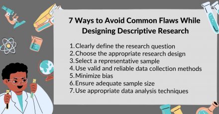
1. Clearly define the research question

A clearly defined research question is the foundation of any research study, and it is important to ensure that the question is both specific and relevant to the topic being studied.

2. Choose the appropriate research design

Choosing the appropriate research design for a study is crucial to the success of the study. Moreover, researchers should choose a design that best fits the research question and the type of data needed to answer it.

3. Select a representative sample

Selecting a representative sample is important to ensure that the findings of the study are generalizable to the population being studied. Researchers should use a sampling method that provides a random and representative sample of the population.

4. Use valid and reliable data collection methods

Using valid and reliable data collection methods is important to ensure that the data collected is accurate and can be used to answer the research question. Researchers should choose methods that are appropriate for the study and that can be administered consistently and systematically.

5. Minimize bias

Bias can significantly impact the validity and reliability of research findings.  Furthermore, it is important to minimize bias in all aspects of the study, from the selection of participants to the analysis of data.

6. Ensure adequate sample size

An adequate sample size is important to ensure that the results of the study are statistically significant and can be generalized to the population being studied.

7. Use appropriate data analysis techniques

The appropriate data analysis technique depends on the type of data collected and the research question being asked. Researchers should choose techniques that are appropriate for the data and the question being asked.

Have you worked on descriptive research designs? How was your experience creating a descriptive design? What challenges did you face? Do write to us or leave a comment below and share your insights on descriptive research designs!

extremely very educative

Indeed very educative and useful. Well explained. Thank you

Simple,easy to understand

Excellent and easy to understand queries and questions get answered easily. Its rather clear than any confusion. Thanks a million Shritika Sirisilla.

Easy to understand. Well written , educative and informative

Rate this article Cancel Reply

Your email address will not be published.

Enago Academy's Most Popular Articles

• Promoting Research

Graphical Abstracts Vs. Infographics: Best practices for using visual illustrations for increased research impact

Dr. Sarah Chen stared at her computer screen, her eyes staring at her recently published…

• Publishing Research

10 Tips to Prevent Research Papers From Being Retracted

Research paper retractions represent a critical event in the scientific community. When a published article…

• Industry News

Google Releases 2024 Scholar Metrics, Evaluates Impact of Scholarly Articles

Google has released its 2024 Scholar Metrics, assessing scholarly articles from 2019 to 2023. This…

Ensuring Academic Integrity and Transparency in Academic Research: A comprehensive checklist for researchers

Academic integrity is the foundation upon which the credibility and value of scientific findings are…

• Reporting Research

How to Optimize Your Research Process: A step-by-step guide

For researchers across disciplines, the path to uncovering novel findings and insights is often filled…

Choosing the Right Analytical Approach: Thematic analysis vs. content analysis for…

Comparing Cross Sectional and Longitudinal Studies: 5 steps for choosing the right…

Research Recommendations – Guiding policy-makers for evidence-based decision making

Sign-up to read more

Subscribe for free to get unrestricted access to all our resources on research writing and academic publishing including:

• 2000+ blog articles
• 50+ Webinars
• 10+ Expert podcasts
• 50+ Infographics
• 10+ Checklists
• Research Guides

We hate spam too. We promise to protect your privacy and never spam you.

• AI in Academia
• Career Corner
• Diversity and Inclusion
• Infographics
• Expert Video Library
• Other Resources
• Enago Learn
• Upcoming & On-Demand Webinars
• Peer Review Week 2024
• Open Access Week 2023
• Conference Videos
• Enago Report
• Journal Finder
• Enago Plagiarism & AI Grammar Check
• Editing Services
• Publication Support Services
• Research Impact
• Translation Services
• Publication solutions
• AI-Based Solutions
• Thought Leadership
• Call for Articles
• Call for Speakers
• Author Training
• Edit Profile

I am looking for Editing/ Proofreading services for my manuscript Tentative date of next journal submission:

Which among these features would you prefer the most in a peer review assistant?

Quant Analysis 101: Descriptive Statistics

Everything You Need To Get Started (With Examples)

By: Derek Jansen (MBA) | Reviewers: Kerryn Warren (PhD) | October 2023

If you’re new to quantitative data analysis , one of the first terms you’re likely to hear being thrown around is descriptive statistics. In this post, we’ll unpack the basics of descriptive statistics, using straightforward language and loads of examples . So grab a cup of coffee and let’s crunch some numbers!

Overview: Descriptive Statistics

What are descriptive statistics.

• Descriptive vs inferential statistics
• Why the descriptives matter
• The “ Big 7 ” descriptive statistics
• Key takeaways

At the simplest level, descriptive statistics summarise and describe relatively basic but essential features of a quantitative dataset – for example, a set of survey responses. They provide a snapshot of the characteristics of your dataset and allow you to better understand, roughly, how the data are “shaped” (more on this later). For example, a descriptive statistic could include the proportion of males and females within a sample or the percentages of different age groups within a population.

Another common descriptive statistic is the humble average (which in statistics-talk is called the mean ). For example, if you undertook a survey and asked people to rate their satisfaction with a particular product on a scale of 1 to 10, you could then calculate the average rating. This is a very basic statistic, but as you can see, it gives you some idea of how this data point is shaped .

What about inferential statistics?

Now, you may have also heard the term inferential statistics being thrown around, and you’re probably wondering how that’s different from descriptive statistics. Simply put, descriptive statistics describe and summarise the sample itself , while inferential statistics use the data from a sample to make inferences or predictions about a population .

Put another way, descriptive statistics help you understand your dataset , while inferential statistics help you make broader statements about the population , based on what you observe within the sample. If you’re keen to learn more, we cover inferential stats in another post , or you can check out the explainer video below.

Why do descriptive statistics matter?

While descriptive statistics are relatively simple from a mathematical perspective, they play a very important role in any research project . All too often, students skim over the descriptives and run ahead to the seemingly more exciting inferential statistics, but this can be a costly mistake.

The reason for this is that descriptive statistics help you, as the researcher, comprehend the key characteristics of your sample without getting lost in vast amounts of raw data. In doing so, they provide a foundation for your quantitative analysis . Additionally, they enable you to quickly identify potential issues within your dataset – for example, suspicious outliers, missing responses and so on. Just as importantly, descriptive statistics inform the decision-making process when it comes to choosing which inferential statistics you’ll run, as each inferential test has specific requirements regarding the shape of the data.

Long story short, it’s essential that you take the time to dig into your descriptive statistics before looking at more “advanced” inferentials. It’s also worth noting that, depending on your research aims and questions, descriptive stats may be all that you need in any case . So, don’t discount the descriptives! 

The “Big 7” descriptive statistics

With the what and why out of the way, let’s take a look at the most common descriptive statistics. Beyond the counts, proportions and percentages we mentioned earlier, we have what we call the “Big 7” descriptives. These can be divided into two categories – measures of central tendency and measures of dispersion.

Measures of central tendency

True to the name, measures of central tendency describe the centre or “middle section” of a dataset. In other words, they provide some indication of what a “typical” data point looks like within a given dataset. The three most common measures are:

The mean , which is the mathematical average of a set of numbers – in other words, the sum of all numbers divided by the count of all numbers. 

The median , which is the middlemost number in a set of numbers, when those numbers are ordered from lowest to highest.

The mode , which is the most frequently occurring number in a set of numbers (in any order). Naturally, a dataset can have one mode, no mode (no number occurs more than once) or multiple modes.

To make this a little more tangible, let’s look at a sample dataset, along with the corresponding mean, median and mode. This dataset reflects the service ratings (on a scale of 1 – 10) from 15 customers.

As you can see, the mean of 5.8 is the average rating across all 15 customers. Meanwhile, 6 is the median . In other words, if you were to list all the responses in order from low to high, Customer 8 would be in the middle (with their service rating being 6). Lastly, the number 5 is the most frequent rating (appearing 3 times), making it the mode.

Together, these three descriptive statistics give us a quick overview of how these customers feel about the service levels at this business. In other words, most customers feel rather lukewarm and there’s certainly room for improvement. From a more statistical perspective, this also means that the data tend to cluster around the 5-6 mark , since the mean and the median are fairly close to each other.

To take this a step further, let’s look at the frequency distribution of the responses . In other words, let’s count how many times each rating was received, and then plot these counts onto a bar chart.

As you can see, the responses tend to cluster toward the centre of the chart , creating something of a bell-shaped curve. In statistical terms, this is called a normal distribution .

As you delve into quantitative data analysis, you’ll find that normal distributions are very common , but they’re certainly not the only type of distribution. In some cases, the data can lean toward the left or the right of the chart (i.e., toward the low end or high end). This lean is reflected by a measure called skewness , and it’s important to pay attention to this when you’re analysing your data, as this will have an impact on what types of inferential statistics you can use on your dataset.

Measures of dispersion

While the measures of central tendency provide insight into how “centred” the dataset is, it’s also important to understand how dispersed that dataset is . In other words, to what extent the data cluster toward the centre – specifically, the mean. In some cases, the majority of the data points will sit very close to the centre, while in other cases, they’ll be scattered all over the place. Enter the measures of dispersion, of which there are three:

Range , which measures the difference between the largest and smallest number in the dataset. In other words, it indicates how spread out the dataset really is.

Variance , which measures how much each number in a dataset varies from the mean (average). More technically, it calculates the average of the squared differences between each number and the mean. A higher variance indicates that the data points are more spread out , while a lower variance suggests that the data points are closer to the mean.

Standard deviation , which is the square root of the variance . It serves the same purposes as the variance, but is a bit easier to interpret as it presents a figure that is in the same unit as the original data . You’ll typically present this statistic alongside the means when describing the data in your research.

Again, let’s look at our sample dataset to make this all a little more tangible.

As you can see, the range of 8 reflects the difference between the highest rating (10) and the lowest rating (2). The standard deviation of 2.18 tells us that on average, results within the dataset are 2.18 away from the mean (of 5.8), reflecting a relatively dispersed set of data .

For the sake of comparison, let’s look at another much more tightly grouped (less dispersed) dataset.

As you can see, all the ratings lay between 5 and 8 in this dataset, resulting in a much smaller range, variance and standard deviation . You might also notice that the data are clustered toward the right side of the graph – in other words, the data are skewed. If we calculate the skewness for this dataset, we get a result of -0.12, confirming this right lean.

In summary, range, variance and standard deviation all provide an indication of how dispersed the data are . These measures are important because they help you interpret the measures of central tendency within context . In other words, if your measures of dispersion are all fairly high numbers, you need to interpret your measures of central tendency with some caution , as the results are not particularly centred. Conversely, if the data are all tightly grouped around the mean (i.e., low dispersion), the mean becomes a much more “meaningful” statistic).

Key Takeaways

We’ve covered quite a bit of ground in this post. Here are the key takeaways:

• Descriptive statistics, although relatively simple, are a critically important part of any quantitative data analysis.
• Measures of central tendency include the mean (average), median and mode.
• Skewness indicates whether a dataset leans to one side or another
• Measures of dispersion include the range, variance and standard deviation

If you’d like hands-on help with your descriptive statistics (or any other aspect of your research project), check out our private coaching service , where we hold your hand through each step of the research journey. 

Psst… there’s more!

This post is an extract from our bestselling short course, Methodology Bootcamp . If you want to work smart, you don't want to miss this .

Good day. May I ask about where I would be able to find the statistics cheat sheet?

Right above you comment 🙂

Good job. you saved me

Brilliant and well explained. So much information explained clearly!

Submit a Comment Cancel reply

Your email address will not be published. Required fields are marked *

Save my name, email, and website in this browser for the next time I comment.

• Print Friendly

Child Care and Early Education Research Connections

Descriptive research studies.

Descriptive research is a type of research that is used to describe the characteristics of a population. It collects data that are used to answer a wide range of what, when, and how questions pertaining to a particular population or group. For example, descriptive studies might be used to answer questions such as: What percentage of Head Start teachers have a bachelor's degree or higher? What is the average reading ability of 5-year-olds when they first enter kindergarten? What kinds of math activities are used in early childhood programs? When do children first receive regular child care from someone other than their parents? When are children with developmental disabilities first diagnosed and when do they first receive services? What factors do programs consider when making decisions about the type of assessments that will be used to assess the skills of the children in their programs? How do the types of services children receive from their early childhood program change as children age?

Descriptive research does not answer questions about why a certain phenomenon occurs or what the causes are. Answers to such questions are best obtained from  randomized and quasi-experimental studies . However, data from descriptive studies can be used to examine the relationships (correlations) among variables. While the findings from correlational analyses are not evidence of causality, they can help to distinguish variables that may be important in explaining a phenomenon from those that are not. Thus, descriptive research is often used to generate hypotheses that should be tested using more rigorous designs.

A variety of data collection methods may be used alone or in combination to answer the types of questions guiding descriptive research. Some of the more common methods include surveys, interviews, observations, case studies, and portfolios. The data collected through these methods can be either quantitative or qualitative. Quantitative data are typically analyzed and presenting using  descriptive statistics . Using quantitative data, researchers may describe the characteristics of a sample or population in terms of percentages (e.g., percentage of population that belong to different racial/ethnic groups, percentage of low-income families that receive different government services) or averages (e.g., average household income, average scores of reading, mathematics and language assessments). Quantitative data, such as narrative data collected as part of a case study, may be used to organize, classify, and used to identify patterns of behaviors, attitudes, and other characteristics of groups.

Descriptive studies have an important role in early care and education research. Studies such as the  National Survey of Early Care and Education  and the  National Household Education Surveys Program  have greatly increased our knowledge of the supply of and demand for child care in the U.S. The  Head Start Family and Child Experiences Survey  and the  Early Childhood Longitudinal Study Program  have provided researchers, policy makers and practitioners with rich information about school readiness skills of children in the U.S.

Each of the methods used to collect descriptive data have their own strengths and limitations. The following are some of the strengths and limitations of descriptive research studies in general.

Study participants are questioned or observed in a natural setting (e.g., their homes, child care or educational settings).

Study data can be used to identify the prevalence of particular problems and the need for new or additional services to address these problems.

Descriptive research may identify areas in need of additional research and relationships between variables that require future study. Descriptive research is often referred to as "hypothesis generating research."

Depending on the data collection method used, descriptive studies can generate rich datasets on large and diverse samples.

Limitations:

Descriptive studies cannot be used to establish cause and effect relationships.

Respondents may not be truthful when answering survey questions or may give socially desirable responses.

The choice and wording of questions on a questionnaire may influence the descriptive findings.

Depending on the type and size of sample, the findings may not be generalizable or produce an accurate description of the population of interest.

Instant insights, infinite possibilities

• What is descriptive research?

Last updated

5 February 2023

Reviewed by

Cathy Heath

Short on time? Get an AI generated summary of this article instead

Descriptive research is a common investigatory model used by researchers in various fields, including social sciences, linguistics, and academia.

Read on to understand the characteristics of descriptive research and explore its underlying techniques, processes, and procedures.

Analyze your descriptive research

Dovetail streamlines analysis to help you uncover and share actionable insights

Descriptive research is an exploratory research method. It enables researchers to precisely and methodically describe a population, circumstance, or phenomenon.

As the name suggests, descriptive research describes the characteristics of the group, situation, or phenomenon being studied without manipulating variables or testing hypotheses . This can be reported using surveys , observational studies, and case studies. You can use both quantitative and qualitative methods to compile the data.

Besides making observations and then comparing and analyzing them, descriptive studies often develop knowledge concepts and provide solutions to critical issues. It always aims to answer how the event occurred, when it occurred, where it occurred, and what the problem or phenomenon is.

• Characteristics of descriptive research

The following are some of the characteristics of descriptive research:

Quantitativeness

Descriptive research can be quantitative as it gathers quantifiable data to statistically analyze a population sample. These numbers can show patterns, connections, and trends over time and can be discovered using surveys, polls, and experiments.

Qualitativeness

Descriptive research can also be qualitative. It gives meaning and context to the numbers supplied by quantitative descriptive research .

Researchers can use tools like interviews, focus groups, and ethnographic studies to illustrate why things are what they are and help characterize the research problem. This is because it’s more explanatory than exploratory or experimental research.

Uncontrolled variables

Descriptive research differs from experimental research in that researchers cannot manipulate the variables. They are recognized, scrutinized, and quantified instead. This is one of its most prominent features.

Cross-sectional studies

Descriptive research is a cross-sectional study because it examines several areas of the same group. It involves obtaining data on multiple variables at the personal level during a certain period. It’s helpful when trying to understand a larger community’s habits or preferences.

Carried out in a natural environment

Descriptive studies are usually carried out in the participants’ everyday environment, which allows researchers to avoid influencing responders by collecting data in a natural setting. You can use online surveys or survey questions to collect data or observe.

Basis for further research

You can further dissect descriptive research’s outcomes and use them for different types of investigation. The outcomes also serve as a foundation for subsequent investigations and can guide future studies. For example, you can use the data obtained in descriptive research to help determine future research designs.

• Descriptive research methods

There are three basic approaches for gathering data in descriptive research: observational, case study, and survey.

You can use surveys to gather data in descriptive research. This involves gathering information from many people using a questionnaire and interview .

Surveys remain the dominant research tool for descriptive research design. Researchers can conduct various investigations and collect multiple types of data (quantitative and qualitative) using surveys with diverse designs.

You can conduct surveys over the phone, online, or in person. Your survey might be a brief interview or conversation with a set of prepared questions intended to obtain quick information from the primary source.

Observation

This descriptive research method involves observing and gathering data on a population or phenomena without manipulating variables. It is employed in psychology, market research , and other social science studies to track and understand human behavior.

Observation is an essential component of descriptive research. It entails gathering data and analyzing it to see whether there is a relationship between the two variables in the study. This strategy usually allows for both qualitative and quantitative data analysis.

Case studies

A case study can outline a specific topic’s traits. The topic might be a person, group, event, or organization.

It involves using a subset of a larger group as a sample to characterize the features of that larger group.

You can generalize knowledge gained from studying a case study to benefit a broader audience.

This approach entails carefully examining a particular group, person, or event over time. You can learn something new about the study topic by using a small group to better understand the dynamics of the entire group.

• Types of descriptive research

There are several types of descriptive study. The most well-known include cross-sectional studies, census surveys, sample surveys, case reports, and comparison studies.

Case reports and case series

In the healthcare and medical fields, a case report is used to explain a patient’s circumstances when suffering from an uncommon illness or displaying certain symptoms. Case reports and case series are both collections of related cases. They have aided the advancement of medical knowledge on countless occasions.

The normative component is an addition to the descriptive survey. In the descriptive–normative survey, you compare the study’s results to the norm.

Descriptive survey

This descriptive type of research employs surveys to collect information on various topics. This data aims to determine the degree to which certain conditions may be attained.

You can extrapolate or generalize the information you obtain from sample surveys to the larger group being researched.

Correlative survey

Correlative surveys help establish if there is a positive, negative, or neutral connection between two variables.

Performing census surveys involves gathering relevant data on several aspects of a given population. These units include individuals, families, organizations, objects, characteristics, and properties.

During descriptive research, you gather different degrees of interest over time from a specific population. Cross-sectional studies provide a glimpse of a phenomenon’s prevalence and features in a population. There are no ethical challenges with them and they are quite simple and inexpensive to carry out.

Comparative studies

These surveys compare the two subjects’ conditions or characteristics. The subjects may include research variables, organizations, plans, and people.

Comparison points, assumption of similarities, and criteria of comparison are three important variables that affect how well and accurately comparative studies are conducted.

For instance, descriptive research can help determine how many CEOs hold a bachelor’s degree and what proportion of low-income households receive government help.

• Pros and cons

The primary advantage of descriptive research designs is that researchers can create a reliable and beneficial database for additional study. To conduct any inquiry, you need access to reliable information sources that can give you a firm understanding of a situation.

Quantitative studies are time- and resource-intensive, so knowing the hypotheses viable for testing is crucial. The basic overview of descriptive research provides helpful hints as to which variables are worth quantitatively examining. This is why it’s employed as a precursor to quantitative research designs.

Some experts view this research as untrustworthy and unscientific. However, there is no way to assess the findings because you don’t manipulate any variables statistically.

Cause-and-effect correlations also can’t be established through descriptive investigations. Additionally, observational study findings cannot be replicated, which prevents a review of the findings and their replication.

The absence of statistical and in-depth analysis and the rather superficial character of the investigative procedure are drawbacks of this research approach.

• Descriptive research examples and applications

Several descriptive research examples are emphasized based on their types, purposes, and applications. Research questions often begin with “What is …” These studies help find solutions to practical issues in social science, physical science, and education.

Here are some examples and applications of descriptive research:

Determining consumer perception and behavior

Organizations use descriptive research designs to determine how various demographic groups react to a certain product or service.

For example, a business looking to sell to its target market should research the market’s behavior first. When researching human behavior in response to a cause or event, the researcher pays attention to the traits, actions, and responses before drawing a conclusion.

Scientific classification

Scientific descriptive research enables the classification of organisms and their traits and constituents.

Measuring data trends

A descriptive study design’s statistical capabilities allow researchers to track data trends over time. It’s frequently used to determine the study target’s current circumstances and underlying patterns.

Conduct comparison

Organizations can use a descriptive research approach to learn how various demographics react to a certain product or service. For example, you can study how the target market responds to a competitor’s product and use that information to infer their behavior.

• Bottom line

A descriptive research design is suitable for exploring certain topics and serving as a prelude to larger quantitative investigations. It provides a comprehensive understanding of the “what” of the group or thing you’re investigating.

This research type acts as the cornerstone of other research methodologies . It is distinctive because it can use quantitative and qualitative research approaches at the same time.

What is descriptive research design?

Descriptive research design aims to systematically obtain information to describe a phenomenon, situation, or population. More specifically, it helps answer the what, when, where, and how questions regarding the research problem rather than the why.

How does descriptive research compare to qualitative research?

Despite certain parallels, descriptive research concentrates on describing phenomena, while qualitative research aims to understand people better.

How do you analyze descriptive research data?

Data analysis involves using various methodologies, enabling the researcher to evaluate and provide results regarding validity and reliability.

Should you be using a customer insights hub?

Do you want to discover previous research faster?

Do you share your research findings with others?

Do you analyze research data?

Start for free today, add your research, and get to key insights faster

Editor’s picks

Last updated: 18 April 2023

Last updated: 27 February 2023

Last updated: 22 August 2024

Last updated: 5 February 2023

Last updated: 16 August 2024

Last updated: 9 March 2023

Last updated: 30 April 2024

Last updated: 12 December 2023

Last updated: 11 March 2024

Last updated: 4 July 2024

Last updated: 6 March 2024

Last updated: 5 March 2024

Last updated: 13 May 2024

Latest articles

Related topics, .css-je19u9{-webkit-align-items:flex-end;-webkit-box-align:flex-end;-ms-flex-align:flex-end;align-items:flex-end;display:-webkit-box;display:-webkit-flex;display:-ms-flexbox;display:flex;-webkit-flex-direction:row;-ms-flex-direction:row;flex-direction:row;-webkit-box-flex-wrap:wrap;-webkit-flex-wrap:wrap;-ms-flex-wrap:wrap;flex-wrap:wrap;-webkit-box-pack:center;-ms-flex-pack:center;-webkit-justify-content:center;justify-content:center;row-gap:0;text-align:center;max-width:671px;}@media (max-width: 1079px){.css-je19u9{max-width:400px;}.css-je19u9>span{white-space:pre;}}@media (max-width: 799px){.css-je19u9{max-width:400px;}.css-je19u9>span{white-space:pre;}} decide what to .css-1kiodld{max-height:56px;display:-webkit-box;display:-webkit-flex;display:-ms-flexbox;display:flex;-webkit-align-items:center;-webkit-box-align:center;-ms-flex-align:center;align-items:center;}@media (max-width: 1079px){.css-1kiodld{display:none;}} build next, decide what to build next, log in or sign up.

Get started for free

• Privacy Policy

Home » Descriptive Analytics – Methods, Tools and Examples

Descriptive Analytics – Methods, Tools and Examples

Table of Contents

Descriptive Analytics

Definition:

Descriptive analytics focused on describing or summarizing raw data and making it interpretable. This type of analytics provides insight into what has happened in the past. It involves the analysis of historical data to identify patterns, trends, and insights. Descriptive analytics often uses visualization tools to represent the data in a way that is easy to interpret.

Descriptive Analytics in Research

Descriptive analytics plays a crucial role in research, helping investigators understand and describe the data collected in their studies. Here’s how descriptive analytics is typically used in a research setting:

• Descriptive Statistics: In research, descriptive analytics often takes the form of descriptive statistics . This includes calculating measures of central tendency (like mean, median, and mode), measures of dispersion (like range, variance, and standard deviation), and measures of frequency (like count, percent, and frequency). These calculations help researchers summarize and understand their data.
• Visualizing Data: Descriptive analytics also involves creating visual representations of data to better understand and communicate research findings . This might involve creating bar graphs, line graphs, pie charts, scatter plots, box plots, and other visualizations.
• Exploratory Data Analysis: Before conducting any formal statistical tests, researchers often conduct an exploratory data analysis, which is a form of descriptive analytics. This might involve looking at distributions of variables, checking for outliers, and exploring relationships between variables.
• Initial Findings: Descriptive analytics are often reported in the results section of a research study to provide readers with an overview of the data. For example, a researcher might report average scores, demographic breakdowns, or the percentage of participants who endorsed each response on a survey.
• Establishing Patterns and Relationships: Descriptive analytics helps in identifying patterns, trends, or relationships in the data, which can guide subsequent analysis or future research. For instance, researchers might look at the correlation between variables as a part of descriptive analytics.

Descriptive Analytics Techniques

Descriptive analytics involves a variety of techniques to summarize, interpret, and visualize historical data. Some commonly used techniques include:

Statistical Analysis

This includes basic statistical methods like mean, median, mode (central tendency), standard deviation, variance (dispersion), correlation, and regression (relationships between variables).

Data Aggregation

It is the process of compiling and summarizing data to obtain a general perspective. It can involve methods like sum, count, average, min, max, etc., often applied to a group of data.

Data Mining

This involves analyzing large volumes of data to discover patterns, trends, and insights. Techniques used in data mining can include clustering (grouping similar data), classification (assigning data into categories), association rules (finding relationships between variables), and anomaly detection (identifying outliers).

Data Visualization

This involves presenting data in a graphical or pictorial format to provide clear and easy understanding of the data patterns, trends, and insights. Common data visualization methods include bar charts, line graphs, pie charts, scatter plots, histograms, and more complex forms like heat maps and interactive dashboards.

This involves organizing data into informational summaries to monitor how different areas of a business are performing. Reports can be generated manually or automatically and can be presented in tables, graphs, or dashboards.

Cross-tabulation (or Pivot Tables)

It involves displaying the relationship between two or more variables in a tabular form. It can provide a deeper understanding of the data by allowing comparisons and revealing patterns and correlations that may not be readily apparent in raw data.

Descriptive Modeling

Some techniques use complex algorithms to interpret data. Examples include decision tree analysis, which provides a graphical representation of decision-making situations, and neural networks, which are used to identify correlations and patterns in large data sets.

Descriptive Analytics Tools

Some common Descriptive Analytics Tools are as follows:

Excel: Microsoft Excel is a widely used tool that can be used for simple descriptive analytics. It has powerful statistical and data visualization capabilities. Pivot tables are a particularly useful feature for summarizing and analyzing large data sets.

Tableau: Tableau is a data visualization tool that is used to represent data in a graphical or pictorial format. It can handle large data sets and allows for real-time data analysis.

Power BI: Power BI, another product from Microsoft, is a business analytics tool that provides interactive visualizations with self-service business intelligence capabilities.

QlikView: QlikView is a data visualization and discovery tool. It allows users to analyze data and use this data to support decision-making.

SAS: SAS is a software suite that can mine, alter, manage and retrieve data from a variety of sources and perform statistical analysis on it.

SPSS: SPSS (Statistical Package for the Social Sciences) is a software package used for statistical analysis. It’s widely used in social sciences research but also in other industries.

Google Analytics: For web data, Google Analytics is a popular tool. It allows businesses to analyze in-depth detail about the visitors on their website, providing valuable insights that can help shape the success strategy of a business.

R and Python: Both are programming languages that have robust capabilities for statistical analysis and data visualization. With packages like pandas, matplotlib, seaborn in Python and ggplot2, dplyr in R, these languages are powerful tools for descriptive analytics.

Looker: Looker is a modern data platform that can take data from any database and let you start exploring and visualizing.

When to use Descriptive Analytics

Descriptive analytics forms the base of the data analysis workflow and is typically the first step in understanding your business or organization’s data. Here are some situations when you might use descriptive analytics:

Understanding Past Behavior: Descriptive analytics is essential for understanding what has happened in the past. If you need to understand past sales trends, customer behavior, or operational performance, descriptive analytics is the tool you’d use.

Reporting Key Metrics: Descriptive analytics is used to establish and report key performance indicators (KPIs). It can help in tracking and presenting these KPIs in dashboards or regular reports.

Identifying Patterns and Trends: If you need to identify patterns or trends in your data, descriptive analytics can provide these insights. This might include identifying seasonality in sales data, understanding peak operational times, or spotting trends in customer behavior.

Informing Business Decisions: The insights provided by descriptive analytics can inform business strategy and decision-making. By understanding what has happened in the past, you can make more informed decisions about what steps to take in the future.

Benchmarking Performance: Descriptive analytics can be used to compare current performance against historical data. This can be used for benchmarking and setting performance goals.

Auditing and Regulatory Compliance: In sectors where compliance and auditing are essential, descriptive analytics can provide the necessary data and trends over specific periods.

Initial Data Exploration: When you first acquire a dataset, descriptive analytics is useful to understand the structure of the data, the relationships between variables, and any apparent anomalies or outliers.

Examples of Descriptive Analytics

Examples of Descriptive Analytics are as follows:

Retail Industry: A retail company might use descriptive analytics to analyze sales data from the past year. They could break down sales by month to identify any seasonality trends. For example, they might find that sales increase in November and December due to holiday shopping. They could also break down sales by product to identify which items are the most popular. This analysis could inform their purchasing and stocking decisions for the next year. Additionally, data on customer demographics could be analyzed to understand who their primary customers are, guiding their marketing strategies.

Healthcare Industry: In healthcare, descriptive analytics could be used to analyze patient data over time. For instance, a hospital might analyze data on patient admissions to identify trends in admission rates. They might find that admissions for certain conditions are higher at certain times of the year. This could help them allocate resources more effectively. Also, analyzing patient outcomes data can help identify the most effective treatments or highlight areas where improvement is needed.

Finance Industry: A financial firm might use descriptive analytics to analyze historical market data. They could look at trends in stock prices, trading volume, or economic indicators to inform their investment decisions. For example, analyzing the price-earnings ratios of stocks in a certain sector over time could reveal patterns that suggest whether the sector is currently overvalued or undervalued. Similarly, credit card companies can analyze transaction data to detect any unusual patterns, which could be signs of fraud.

Advantages of Descriptive Analytics

Descriptive analytics plays a vital role in the world of data analysis, providing numerous advantages:

• Understanding the Past: Descriptive analytics provides an understanding of what has happened in the past, offering valuable context for future decision-making.
• Data Summarization: Descriptive analytics is used to simplify and summarize complex datasets, which can make the information more understandable and accessible.
• Identifying Patterns and Trends: With descriptive analytics, organizations can identify patterns, trends, and correlations in their data, which can provide valuable insights.
• Inform Decision-Making: The insights generated through descriptive analytics can inform strategic decisions and help organizations to react more quickly to events or changes in behavior.
• Basis for Further Analysis: Descriptive analytics lays the groundwork for further analytical activities. It’s the first necessary step before moving on to more advanced forms of analytics like predictive analytics (forecasting future events) or prescriptive analytics (advising on possible outcomes).
• Performance Evaluation: It allows organizations to evaluate their performance by comparing current results with past results, enabling them to see where improvements have been made and where further improvements can be targeted.
• Enhanced Reporting and Dashboards: Through the use of visualization techniques, descriptive analytics can improve the quality of reports and dashboards, making the data more understandable and easier to interpret for stakeholders at all levels of the organization.
• Immediate Value: Unlike some other types of analytics, descriptive analytics can provide immediate insights, as it doesn’t require complex models or deep analytical capabilities to provide value.

Disadvantages of Descriptive Analytics

While descriptive analytics offers numerous benefits, it also has certain limitations or disadvantages. Here are a few to consider:

• Limited to Past Data: Descriptive analytics primarily deals with historical data and provides insights about past events. It does not predict future events or trends and can’t help you understand possible future outcomes on its own.
• Lack of Deep Insights: While descriptive analytics helps in identifying what happened, it does not answer why it happened. For deeper insights, you would need to use diagnostic analytics, which analyzes data to understand the root cause of a particular outcome.
• Can Be Misleading: If not properly executed, descriptive analytics can sometimes lead to incorrect conclusions. For example, correlation does not imply causation, but descriptive analytics might tempt one to make such an inference.
• Data Quality Issues: The accuracy and usefulness of descriptive analytics are heavily reliant on the quality of the underlying data. If the data is incomplete, incorrect, or biased, the results of the descriptive analytics will be too.
• Over-reliance on Descriptive Analytics: Businesses may rely too much on descriptive analytics and not enough on predictive and prescriptive analytics. While understanding past and present data is important, it’s equally vital to forecast future trends and make data-driven decisions based on those predictions.
• Doesn’t Provide Actionable Insights: Descriptive analytics is used to interpret historical data and identify patterns and trends, but it doesn’t provide recommendations or courses of action. For that, prescriptive analytics is needed.

About the author

Muhammad Hassan

Researcher, Academic Writer, Web developer

You may also like

What is Data Science? Components, Process and Tools

Social Network Analysis – Types, Tools and...

Digital Ethnography – Types, Methods and Examples

Prescriptive Analytics – Techniques, Tools and...

What is Big Data? Types, Tools and Examples

Emerging Research Methods – Types and Examples

Have a language expert improve your writing

Run a free plagiarism check in 10 minutes, generate accurate citations for free.

• Knowledge Base

Methodology

• Types of Research Designs Compared | Guide & Examples

Types of Research Designs Compared | Guide & Examples

Published on June 20, 2019 by Shona McCombes . Revised on June 22, 2023.

When you start planning a research project, developing research questions and creating a  research design , you will have to make various decisions about the type of research you want to do.

There are many ways to categorize different types of research. The words you use to describe your research depend on your discipline and field. In general, though, the form your research design takes will be shaped by:

• The type of knowledge you aim to produce
• The type of data you will collect and analyze
• The sampling methods , timescale and location of the research

This article takes a look at some common distinctions made between different types of research and outlines the key differences between them.

Table of contents

Types of research aims, types of research data, types of sampling, timescale, and location, other interesting articles.

The first thing to consider is what kind of knowledge your research aims to contribute.

Here's why students love Scribbr's proofreading services

Discover proofreading & editing

The next thing to consider is what type of data you will collect. Each kind of data is associated with a range of specific research methods and procedures.

Finally, you have to consider three closely related questions: how will you select the subjects or participants of the research? When and how often will you collect data from your subjects? And where will the research take place?

Keep in mind that the methods that you choose bring with them different risk factors and types of research bias . Biases aren’t completely avoidable, but can heavily impact the validity and reliability of your findings if left unchecked.

Choosing between all these different research types is part of the process of creating your research design , which determines exactly how your research will be conducted. But the type of research is only the first step: next, you have to make more concrete decisions about your research methods and the details of the study.

Read more about creating a research design

If you want to know more about statistics , methodology , or research bias , make sure to check out some of our other articles with explanations and examples.

• Normal distribution
• Degrees of freedom
• Null hypothesis
• Discourse analysis
• Control groups
• Mixed methods research
• Non-probability sampling
• Quantitative research
• Ecological validity

Research bias

• Rosenthal effect
• Implicit bias
• Cognitive bias
• Selection bias
• Negativity bias
• Status quo bias

Cite this Scribbr article

If you want to cite this source, you can copy and paste the citation or click the “Cite this Scribbr article” button to automatically add the citation to our free Citation Generator.

McCombes, S. (2023, June 22). Types of Research Designs Compared | Guide & Examples. Scribbr. Retrieved September 9, 2024, from https://www.scribbr.com/methodology/types-of-research/

Is this article helpful?

Shona McCombes

Other students also liked, what is a research design | types, guide & examples, qualitative vs. quantitative research | differences, examples & methods, what is a research methodology | steps & tips, "i thought ai proofreading was useless but..".

I've been using Scribbr for years now and I know it's a service that won't disappoint. It does a good job spotting mistakes”

Want to create or adapt books like this? Learn more about how Pressbooks supports open publishing practices.

Descriptive Research and Case Studies

Learning objectives.

• Explain the importance and uses of descriptive research, especially case studies, in studying abnormal behavior

Types of Research Methods

There are many research methods available to psychologists in their efforts to understand, describe, and explain behavior and the cognitive and biological processes that underlie it. Some methods rely on observational techniques. Other approaches involve interactions between the researcher and the individuals who are being studied—ranging from a series of simple questions; to extensive, in-depth interviews; to well-controlled experiments.

The three main categories of psychological research are descriptive, correlational, and experimental research. Research studies that do not test specific relationships between variables are called descriptive, or qualitative, studies . These studies are used to describe general or specific behaviors and attributes that are observed and measured. In the early stages of research, it might be difficult to form a hypothesis, especially when there is not any existing literature in the area. In these situations designing an experiment would be premature, as the question of interest is not yet clearly defined as a hypothesis. Often a researcher will begin with a non-experimental approach, such as a descriptive study, to gather more information about the topic before designing an experiment or correlational study to address a specific hypothesis. Descriptive research is distinct from correlational research , in which psychologists formally test whether a relationship exists between two or more variables. Experimental research goes a step further beyond descriptive and correlational research and randomly assigns people to different conditions, using hypothesis testing to make inferences about how these conditions affect behavior. It aims to determine if one variable directly impacts and causes another. Correlational and experimental research both typically use hypothesis testing, whereas descriptive research does not.

Each of these research methods has unique strengths and weaknesses, and each method may only be appropriate for certain types of research questions. For example, studies that rely primarily on observation produce incredible amounts of information, but the ability to apply this information to the larger population is somewhat limited because of small sample sizes. Survey research, on the other hand, allows researchers to easily collect data from relatively large samples. While surveys allow results to be generalized to the larger population more easily, the information that can be collected on any given survey is somewhat limited and subject to problems associated with any type of self-reported data. Some researchers conduct archival research by using existing records. While existing records can be a fairly inexpensive way to collect data that can provide insight into a number of research questions, researchers using this approach have no control on how or what kind of data was collected.

Correlational research can find a relationship between two variables, but the only way a researcher can claim that the relationship between the variables is cause and effect is to perform an experiment. In experimental research, which will be discussed later, there is a tremendous amount of control over variables of interest. While performing an experiment is a powerful approach, experiments are often conducted in very artificial settings, which calls into question the validity of experimental findings with regard to how they would apply in real-world settings. In addition, many of the questions that psychologists would like to answer cannot be pursued through experimental research because of ethical concerns.

The three main types of descriptive studies are case studies, naturalistic observation, and surveys.

Clinical or Case Studies

Psychologists can use a detailed description of one person or a small group based on careful observation.  Case studies  are intensive studies of individuals and have commonly been seen as a fruitful way to come up with hypotheses and generate theories. Case studies add descriptive richness. Case studies are also useful for formulating concepts, which are an important aspect of theory construction. Through fine-grained knowledge and description, case studies can fully specify the causal mechanisms in a way that may be harder in a large study.

Sigmund Freud   developed  many theories from case studies (Anna O., Little Hans, Wolf Man, Dora, etc.). F or example, he conducted a case study of a man, nicknamed “Rat Man,”  in which he claimed that this patient had been cured by psychoanalysis.  T he nickname derives from the fact that among the patient’s many compulsions, he had an obsession with nightmarish fantasies about rats. 

Today, more commonly, case studies reflect an up-close, in-depth, and detailed examination of an individual’s course of treatment. Case studies typically include a complete history of the subject’s background and response to treatment. From the particular client’s experience in therapy, the therapist’s goal is to provide information that may help other therapists who treat similar clients.

Case studies are generally a single-case design, but can also be a multiple-case design, where replication instead of sampling is the criterion for inclusion. Like other research methodologies within psychology, the case study must produce valid and reliable results in order to be useful for the development of future research. Distinct advantages and disadvantages are associated with the case study in psychology.

A commonly described limit of case studies is that they do not lend themselves to generalizability . The other issue is that the case study is subject to the bias of the researcher in terms of how the case is written, and that cases are chosen because they are consistent with the researcher’s preconceived notions, resulting in biased research. Another common problem in case study research is that of reconciling conflicting interpretations of the same case history.

Despite these limitations, there are advantages to using case studies. One major advantage of the case study in psychology is the potential for the development of novel hypotheses of the  cause of abnormal behavior   for later testing. Second, the case study can provide detailed descriptions of specific and rare cases and help us study unusual conditions that occur too infrequently to study with large sample sizes. The major disadvantage is that case studies cannot be used to determine causation, as is the case in experimental research, where the factors or variables hypothesized to play a causal role are manipulated or controlled by the researcher. 

Link to Learning: Famous Case Studies

Some well-known case studies that related to abnormal psychology include the following:

• Harlow— Phineas Gage
• Breuer & Freud (1895)— Anna O.
• Cleckley’s case studies: on psychopathy ( The Mask of Sanity ) (1941) and multiple personality disorder ( The Three Faces of Eve ) (1957)
• Freud and  Little Hans
• Freud and the  Rat Man
• John Money and the  John/Joan case
• Genie (feral child)
• Piaget’s studies
• Rosenthal’s book on the  murder of Kitty Genovese
• Washoe (sign language)
• Patient H.M.

Naturalistic Observation

If you want to understand how behavior occurs, one of the best ways to gain information is to simply observe the behavior in its natural context. However, people might change their behavior in unexpected ways if they know they are being observed. How do researchers obtain accurate information when people tend to hide their natural behavior? As an example, imagine that your professor asks everyone in your class to raise their hand if they always wash their hands after using the restroom. Chances are that almost everyone in the classroom will raise their hand, but do you think hand washing after every trip to the restroom is really that universal?

This is very similar to the phenomenon mentioned earlier in this module: many individuals do not feel comfortable answering a question honestly. But if we are committed to finding out the facts about handwashing, we have other options available to us.

Suppose we send a researcher to a school playground to observe how aggressive or socially anxious children interact with peers. Will our observer blend into the playground environment by wearing a white lab coat, sitting with a clipboard, and staring at the swings? We want our researcher to be inconspicuous and unobtrusively positioned—perhaps pretending to be a school monitor while secretly recording the relevant information. This type of observational study is called naturalistic observation : observing behavior in its natural setting. To better understand peer exclusion, Suzanne Fanger collaborated with colleagues at the University of Texas to observe the behavior of preschool children on a playground. How did the observers remain inconspicuous over the duration of the study? They equipped a few of the children with wireless microphones (which the children quickly forgot about) and observed while taking notes from a distance. Also, the children in that particular preschool (a “laboratory preschool”) were accustomed to having observers on the playground (Fanger, Frankel, & Hazen, 2012).

It is critical that the observer be as unobtrusive and as inconspicuous as possible: when people know they are being watched, they are less likely to behave naturally. For example, psychologists have spent weeks observing the behavior of homeless people on the streets, in train stations, and bus terminals. They try to ensure that their naturalistic observations are unobtrusive, so as to minimize interference with the behavior they observe. Nevertheless, the presence of the observer may distort the behavior that is observed, and this must be taken into consideration (Figure 1).

The greatest benefit of naturalistic observation is the validity, or accuracy, of information collected unobtrusively in a natural setting. Having individuals behave as they normally would in a given situation means that we have a higher degree of ecological validity, or realism, than we might achieve with other research approaches. Therefore, our ability to generalize the findings of the research to real-world situations is enhanced. If done correctly, we need not worry about people modifying their behavior simply because they are being observed. Sometimes, people may assume that reality programs give us a glimpse into authentic human behavior. However, the principle of inconspicuous observation is violated as reality stars are followed by camera crews and are interviewed on camera for personal confessionals. Given that environment, we must doubt how natural and realistic their behaviors are.

The major downside of naturalistic observation is that they are often difficult to set up and control. Although something as simple as observation may seem like it would be a part of all research methods, participant observation is a distinct methodology that involves the researcher embedding themselves into a group in order to study its dynamics. For example, Festinger, Riecken, and Shacter (1956) were very interested in the psychology of a particular cult. However, this cult was very secretive and wouldn’t grant interviews to outside members. So, in order to study these people, Festinger and his colleagues pretended to be cult members, allowing them access to the behavior and psychology of the cult. Despite this example, it should be noted that the people being observed in a participant observation study usually know that the researcher is there to study them. [1]

Another potential problem in observational research is observer bias . Generally, people who act as observers are closely involved in the research project and may unconsciously skew their observations to fit their research goals or expectations. To protect against this type of bias, researchers should have clear criteria established for the types of behaviors recorded and how those behaviors should be classified. In addition, researchers often compare observations of the same event by multiple observers, in order to test inter-rater reliability : a measure of reliability that assesses the consistency of observations by different observers.

Often, psychologists develop surveys as a means of gathering data. Surveys are lists of questions to be answered by research participants, and can be delivered as paper-and-pencil questionnaires, administered electronically, or conducted verbally (Figure 3). Generally, the survey itself can be completed in a short time, and the ease of administering a survey makes it easy to collect data from a large number of people.

Surveys allow researchers to gather data from larger samples than may be afforded by other research methods . A sample is a subset of individuals selected from a population , which is the overall group of individuals that the researchers are interested in. Researchers study the sample and seek to generalize their findings to the population.

There is both strength and weakness in surveys when compared to case studies. By using surveys, we can collect information from a larger sample of people. A larger sample is better able to reflect the actual diversity of the population, thus allowing better generalizability. Therefore, if our sample is sufficiently large and diverse, we can assume that the data we collect from the survey can be generalized to the larger population with more certainty than the information collected through a case study. However, given the greater number of people involved, we are not able to collect the same depth of information on each person that would be collected in a case study.

Another potential weakness of surveys is something we touched on earlier in this module: people do not always give accurate responses. They may lie, misremember, or answer questions in a way that they think makes them look good. For example, people may report drinking less alcohol than is actually the case.

Any number of research questions can be answered through the use of surveys. One real-world example is the research conducted by Jenkins, Ruppel, Kizer, Yehl, and Griffin (2012) about the backlash against the U.S. Arab-American community following the terrorist attacks of September 11, 2001. Jenkins and colleagues wanted to determine to what extent these negative attitudes toward Arab-Americans still existed nearly a decade after the attacks occurred. In one study, 140 research participants filled out a survey with 10 questions, including questions asking directly about the participant’s overt prejudicial attitudes toward people of various ethnicities. The survey also asked indirect questions about how likely the participant would be to interact with a person of a given ethnicity in a variety of settings (such as, “How likely do you think it is that you would introduce yourself to a person of Arab-American descent?”). The results of the research suggested that participants were unwilling to report prejudicial attitudes toward any ethnic group. However, there were significant differences between their pattern of responses to questions about social interaction with Arab-Americans compared to other ethnic groups: they indicated less willingness for social interaction with Arab-Americans compared to the other ethnic groups. This suggested that the participants harbored subtle forms of prejudice against Arab-Americans, despite their assertions that this was not the case (Jenkins et al., 2012).

Think it Over

Research has shown that parental depressive symptoms are linked to a number of negative child outcomes. A classmate of yours is interested in  the associations between parental depressive symptoms and actual child behaviors in everyday life [2] because this associations remains largely unknown. After reading this section, what do you think is the best way to better understand such associations? Which method might result in the most valid data?

clinical or case study:  observational research study focusing on one or a few people

correlational research:  tests whether a relationship exists between two or more variables

descriptive research:  research studies that do not test specific relationships between variables; they are used to describe general or specific behaviors and attributes that are observed and measured

experimental research:  tests a hypothesis to determine cause-and-effect relationships

generalizability:  inferring that the results for a sample apply to the larger population

inter-rater reliability:  measure of agreement among observers on how they record and classify a particular event

naturalistic observation:  observation of behavior in its natural setting

observer bias:  when observations may be skewed to align with observer expectations

population:  overall group of individuals that the researchers are interested in

sample:  subset of individuals selected from the larger population

survey:  list of questions to be answered by research participants—given as paper-and-pencil questionnaires, administered electronically, or conducted verbally—allowing researchers to collect data from a large number of people

CC Licensed Content, Shared Previously

• Descriptive Research and Case Studies . Authored by : Sonja Ann Miller for Lumen Learning.  Provided by : Lumen Learning.  License :  CC BY-SA: Attribution-ShareAlike
• Approaches to Research.  Authored by : OpenStax College.  Located at :  http://cnx.org/contents/[email protected]:iMyFZJzg@5/Approaches-to-Research .  License :  CC BY: Attribution .  License Terms : Download for free at http://cnx.org/contents/[email protected]
• Descriptive Research.  Provided by : Boundless.  Located at :  https://www.boundless.com/psychology/textbooks/boundless-psychology-textbook/researching-psychology-2/types-of-research-studies-27/descriptive-research-124-12659/ .  License :  CC BY-SA: Attribution-ShareAlike
• Case Study.  Provided by : Wikipedia.  Located at :  https://en.wikipedia.org/wiki/Case_study .  License :  CC BY-SA: Attribution-ShareAlike
• Rat man.  Provided by : Wikipedia.  Located at :  https://en.wikipedia.org/wiki/Rat_Man#Legacy .  License :  CC BY-SA: Attribution-ShareAlike
• Case study in psychology.  Provided by : Wikipedia.  Located at :  https://en.wikipedia.org/wiki/Case_study_in_psychology .  License :  CC BY-SA: Attribution-ShareAlike
• Research Designs.  Authored by : Christie Napa Scollon.  Provided by : Singapore Management University.  Located at :  https://nobaproject.com/modules/research-designs#reference-6 .  Project : The Noba Project.  License :  CC BY-NC-SA: Attribution-NonCommercial-ShareAlike
• Single subject design.  Provided by : Wikipedia.  Located at :  https://en.wikipedia.org/wiki/Single-subject_design .  License :  CC BY-SA: Attribution-ShareAlike
• Single subject research.  Provided by : Wikipedia.  Located at :  https://en.wikipedia.org/wiki/Single-subject_research#A-B-A-B .  License :  Public Domain: No Known Copyright
• Pills.  Authored by : qimono.  Provided by : Pixabay.  Located at :  https://pixabay.com/illustrations/pill-capsule-medicine-medical-1884775/ .  License :  CC0: No Rights Reserved
• ABAB Design.  Authored by : Doc. Yu.  Provided by : Wikimedia.  Located at :  https://commons.wikimedia.org/wiki/File:A-B-A-B_Design.png .  License :  CC BY-SA: Attribution-ShareAlike
• Scollon, C. N. (2020). Research designs. In R. Biswas-Diener & E. Diener (Eds), Noba textbook series: Psychology. Champaign, IL: DEF publishers. Retrieved from http://noba.to/acxb2thy ↵
• Slatcher, R. B., & Trentacosta, C. J. (2011). A naturalistic observation study of the links between parental depressive symptoms and preschoolers' behaviors in everyday life. Journal of family psychology : JFP : journal of the Division of Family Psychology of the American Psychological Association (Division 43), 25(3), 444–448. https://doi.org/10.1037/a0023728 ↵

Descriptive Research and Case Studies Copyright © by Meredith Palm is licensed under a Creative Commons Attribution 4.0 International License , except where otherwise noted.

Share This Book

• Voxco Online
• Voxco Panel Management
• Voxco Panel Portal
• Voxco Audience
• Voxco Mobile Offline
• Voxco Dialer Cloud
• Voxco Dialer On-premise
• Voxco TCPA Connect
• Voxco Analytics
• Voxco Text & Sentiment Analysis

• 40+ question types
• Drag-and-drop interface
• Skip logic and branching
• Multi-lingual survey
• Text piping
• Question library
• CSS customization
• White-label surveys
• Customizable ‘Thank You’ page
• Customizable survey theme
• Reminder send-outs
• Survey rewards
• Social media
• Website surveys
• Correlation analysis
• Cross-tabulation analysis
• Trend analysis
• Real-time dashboard
• Customizable report
• Email address validation
• Recaptcha validation
• SSL security

Take a peek at our powerful survey features to design surveys that scale discoveries.

Download feature sheet.

• Hospitality
• Academic Research
• Customer Experience
• Employee Experience
• Product Experience
• Market Research
• Social Research
• Data Analysis

Explore Voxco 

Need to map Voxco’s features & offerings? We can help!

Watch a Demo 

Download Brochures 

Get a Quote

• NPS Calculator
• CES Calculator
• A/B Testing Calculator
• Margin of Error Calculator
• Sample Size Calculator
• CX Strategy & Management Hub
• Market Research Hub
• Patient Experience Hub
• Employee Experience Hub
• NPS Knowledge Hub
• Market Research Guide
• Customer Experience Guide
• Survey Research Guides
• Survey Template Library
• Webinars and Events
• Feature Sheets
• Try a sample survey
• Professional Services

Get exclusive insights into research trends and best practices from top experts! Access Voxco’s ‘State of Research Report 2024 edition’ .

We’ve been avid users of the Voxco platform now for over 20 years. It gives us the flexibility to routinely enhance our survey toolkit and provides our clients with a more robust dataset and story to tell their clients.

VP Innovation & Strategic Partnerships, The Logit Group

• Client Stories
• Voxco Reviews
• Why Voxco Research?
• Careers at Voxco
• Vulnerabilities and Ethical Hacking

Explore Regional Offices

• Survey Software The world’s leading omnichannel survey software
• Online Survey Tools Create sophisticated surveys with ease.
• Mobile Offline Conduct efficient field surveys.
• Text Analysis
• Close The Loop
• Automated Translations
• NPS Dashboard
• CATI Manage high volume phone surveys efficiently
• Cloud/On-premise Dialer TCPA compliant Cloud on-premise dialer
• IVR Survey Software Boost productivity with automated call workflows.
• Analytics Analyze survey data with visual dashboards
• Panel Manager Nurture a loyal community of respondents.
• Survey Portal Best-in-class user friendly survey portal.
• Voxco Audience Conduct targeted sample research in hours.
• Predictive Analytics
• Customer 360
• Customer Loyalty
• Fraud & Risk Management
• AI/ML Enablement Services
• Credit Underwriting

Find the best survey software for you! (Along with a checklist to compare platforms)

Get Buyer’s Guide

• 100+ question types
• SMS surveys
• Financial Services
• Banking & Financial Services
• Retail Solution
• Risk Management
• Customer Lifecycle Solutions
• Net Promoter Score
• Customer Behaviour Analytics
• Customer Segmentation
• Data Unification

Explore Voxco 

Watch a Demo 

Download Brochures 

• CX Strategy & Management Hub
• The Voxco Guide to Customer Experience
• Professional services
• Blogs & White papers
• Case Studies

Find the best customer experience platform

Uncover customer pain points, analyze feedback and run successful CX programs with the best CX platform for your team.

Get the Guide Now

VP Innovation & Strategic Partnerships, The Logit Group

• Why Voxco Intelligence?
• Our clients
• Client stories
• Featuresheets

Descriptive Research: Definition, Methods & Examples

• August 19, 2021

Voxco’s Descriptive Research guide helps uncover the how, when, what, and where questions in a research problem

SHARE THE ARTICLE ON

When you are a store manager in a convenience store, and you have to make a report. Any finding such as which product is selling most, what time of the day you have the most crowd, or which product customers are demanding most, all these observations and reporting is descriptive research. 

It is often the first step of any research since the data you gather sets the stage for the research question. It is used to determine the problem you want to explore before fully realizing it. The information helps you identify the problem. 

In this blog, we’ll discuss the characteristics, types, pros & cons, and three ways to conduct this research type to help you in your next market research.

What is descriptive research?

Descriptive research refers to the research method that describes the characteristics of the variables you are studying. This methodology focuses on answering questions to the “WHAT” than the “WHY” of the research question. The primary focus of this research method is to describe the nature of the demographics understudy instead of focusing on the “why”.

It is called an observational research method as none of the variables in the study are influenced during the research process.

For example, let’s assume that a UK-based brand is trying to establish itself in New York and wants to understand the demographics of the buyers who generally purchase from brands similar to it. 

In descriptive research, the information gathered from the survey will only focus on the population’s demographics. It will uncover details on the buying patterns of different age cohorts in New York. It will not study why such patterns exist because the brand is trying to establish itself in New York. 

They want to understand the buying behavior of the population, not why such associations exist. It is a part of quantitative market research or social research study, which involves conducting survey research using quantitative variables on a market research software or social research software .

Voxco’s omnichannel survey software helps you collect insights from multiple channels using a single platform.

See the true power of using an integrated survey platform to conduct online, offline, and phone surveys along with a built-in analytical suite.

What are the characteristics of descriptive research?

Among the many, the following are the main characteristics of this research type:

• Quantitative research
• Nature of variables
• Cross-sectional studies
• Directs future research

Let’s discuss these four characteristics in detail. 

1. Quantitative research:

It is quantitative as it attempts to collect and statistically analyze information. This research type is a powerful research tool that permits a researcher to collect data and describe the demographics of the same with the help of statistical analysis. Thus, it is a quantitative research method .

2. Nature of variables:

The variables included in this research are uncontrolled. They are not manipulated in any way. Descriptive research mostly uses observational methods; thus, the researcher cannot control the nature and behavior of the variables under study.

3. Cross-sectional studies:

In this research type, different sections of the same group are studied. For instance, in order to study the fashion preferences of New York, the researcher can study Gen Z as well as Millennials from the same population in New York.

4. Directs future research:

Since this research identifies the patterns between variables and describes them, researchers can further study the data collected here. It guides researchers to discover further why such patterns have been found and their association. Hence, it gives researchers a direction toward insightful market research.

What are the methods of conducting descriptive research?

Primarily, there are three descriptive research methods: 

• Observation,
• Survey, & 

We have explained how you can conduct this research type in three different ways. Each method helps gather descriptive data and sets the scene for thorough research.

1. Observational method

All research has some component of observation, this observation can be quantitative or qualitative. A quantitative observation includes objectively collecting data that is primarily in numerical form. 

The data collected should be related to or understood in terms of quantity.

Quantitative observations are analyzed with the help of survey analytics software . 

Examples of quantitative observations include observation of any variable related to a numerical value such as age, shape, weight, height, scale, etc.

For example, a researcher can understand a customer’s satisfaction with their recent purchases by asking them to rate their satisfaction on a Likert scale ranging from 1 (extremely unsatisfied) to 7 (extremely satisfied).

Qualitative observations monitor the characteristics of a phenomenon and do not involve numerical measurements.

Using this type of descriptive research, you can observe respondents in a naturalistic environment from a distance. Since the respondents are in a natural environment, the observed characteristics enrich and offer more insights. 

For instance, you can monitor and note down the observations of customers in a supermarket by observing their selection and purchasing patterns. This offers a detailed cognizance of the customer.

In any kind of research, you should ensure high survey response rates for improved quality of insights.  

2. Survey method

The survey method includes recording the answers of respondents through surveys or questionnaires. Surveys can include polls as well. They are the most common tool for collecting market research data. 

Surveys are generally used to collect feedback from the respondents. It should have a survey that taps into both open-ended and closed-ended questions .

The biggest advantage of the survey method is that it can be conducted using online or offline survey tools . One of the reasons why the survey method is the go-to option for descriptive research is that it entails the collection of large amounts of data in a limited span of time.

3. Case study method

The in-depth study of an individual or a group is known as a case study. Case studies usually lead to developing a hypothesis to explore a phenomenon further. Case studies are limited in their scope in that they don’t allow the researcher to make cause-effect conclusions or accurate predictions. 

This is because these associations could reflect the bias on the researchers’ part instead of a naturally occurring phenomenon. Another reason why case studies are limited in scope is that they could just be reflecting an atypical respondent in the survey. 

An atypical respondent refers to someone who is different from the average consumer, and if researchers make judgments about the entire target population based on this consumer, it can affect the external validity of the study.

[ Related read: Descriptive vs experimental research ]

Read how Voxco helped Brain Research improve research productivity by 60%.

“The platform extends our ability to productively manage our busy intercept survey projects, and the confidence to support major new clients.”

Laura Ruvalcaba, President & CEO, Brain Research

What are the types of descriptive research?

There are seven types of descriptive research based on when you conduct them and what type of data research you conduct. We have explained these seven types in brief with examples to help you better understand them.

1. Cross-sectional: 

A descriptive method of studying a particular section of the target population at a specific point in time. 

Example : Tracking the use of social media by Gen Z in the Netherlands. 

2. Longitudinal: 

This type of descriptive study is conducted for an extended period on a group of people. 

Example : Monitoring changes in the volume of cyber-bullying among Millenials from 2022 to 2024. 

3. Normative: 

In this descriptive method, we compare the result of a study with an existing norm. 

Example : Comparing legal verdicts in similar types of cases. 

4. Relational/Correlational:

We investigate the type of relationships (correlation) between two variables in this type of descriptive research. 

Example : Investigating the relationship between video games and mental health. 

5. Comparative: 

A descriptive study that compares two or more people, groups, or conditions based on a specific aspect. 

Example : Comparing the salary of two employees in similar job roles from two companies. 

6. Classification: 

This type of research arranges collected data into classes based on specific criteria to analyze them. 

Example : Classification of customers based on their buying behavior. 

7. Archival: 

A descriptive study where you search for past records and extract information.

Example : Tracking company’s sales data over the decade. 

We have been discussing the descriptive method with examples. So now let’s see how you can use this research type in a real-world application.

Guide to Descriptive Research

Learn the key steps of conducting descriptive research to uncover breakthrough insights into your target market.

Examples of Descriptive Research Under Market Research

This research type helps you gather the necessary information you need to understand the problem. It sets the scene to conduct further research. But how can you use this research method in the real world? 

We have explained its real-world application in three scenarios to help you determine where and where you want to use this research type. 

1. Sales Studies

You can use this research type to analyze the potential of the market, what is currently trending in the market, and which products may perform well in terms of sales. You can also study what circumstances influence the market shares and when they are likely to increase or decrease. 

This research type can help you gather the demographic data of the consumers.

2. Consumer Perception and Behavior Studies

You can use this research method to analyze what consumers think about the brand. You can evaluate their perceptions about the products sold by a particular brand and the uses of other competitive products. 

Using descriptive research, you can also analyze what advertising strategies have worked to increase the positive perceptions of the brand. You can assess consumers’ consumption behavior and how it is influenced by product pricing.

3. Market Characteristics Studies

Another way you can use this research method is by analyzing the distribution of the products in the market. You can gather contextual data on questions such as “which countries have more sales”, “which countries have fewer products but the product is sold out quickly” , etc. 

You can also analyze the brand management of competitors ; what strategy is working for them and what is not.

What are the applications of descriptive research?

This research method is used for a variety of reasons. Even after outlining survey goals, and survey designs as well as collecting information through surveys, there is no way of knowing whether or not the research you are conducting will meet the predictions that you have made. 

Here are some popular ways in which organizations use this research type:

1. Defining the characteristics of respondents

Since most descriptive research methods use close-ended questions for the collection of data, it helps in drawing objective conclusions about the respondents.

It helps in deriving patterns, traits, and behaviors of respondents. It also aims to understand respondents’ attitudes and opinions about certain phenomena.

For instance , researchers can understand how many hours young adults spend on the internet, their opinions about social media platforms, and how important they consider these platforms to be. This information will help the company make informed decisions regarding its products and brands. 

One-stop-shop to gather, measure, uncover, and act on insightful data.

Curious about the price? Click below to get a personalized quote.

2. Analyzing trends in data

You can use statistical data analysis to understand the trends in data over time. 

For instance, consider an apparel company that drops a new line of clothing; they may research how Gen Z and Millennials react to the new launch. If they discover that the new range of clothes has worked effectively for one group (Gen Z) but not the other, the company may stop producing clothes for the other group.

Leverage a data analysis platform that allows you to conduct advanced statistical analysis and offers a data analytics dashboard to track real-time data.

3. Comparing different groups

Something closely knit to the previous point is also comparing different groups of customers based on their demographics. With descriptive research, you can study how different groups of people respond to specific services offered by a company. 

For instance , what is the influence of income, age, gender, income, etc. influence the spending behaviors of consumers?

This research method helps companies understand what they should do to increase their brand appeal in different groups of the population. 

4. Validating existing patterns of respondents

Since it is non-invasive and makes use of quantitative data (mostly), you can make observations about why the current patterns of purchasing exist in customers. 

You can also use the findings as the basis of a more in-depth study in the future. 

5. Conducting research at different times

Descriptive research can be conducted at different periods of time in order to see whether the patterns are similar or dissimilar at different points in time. You can also replicate the studies to verify the findings of the original study to draw accurate conclusions.

6. Finding correlations among variables

This method is also used to draw correlations between variables and the degree of association between the variables. 

For instance, if the focus is on men’s age and expenditure. 

There is a possibility of finding a negative correlation between the two variables, indicating that as the age of men increases, the less they spend on sports products.

Descriptive research Examples

A descriptive method of research aims to gather answers for how, what, when, and where. 

Let’s use some examples to understand how a descriptive method of research is used. 

Before investing in housing at any location, you would want to conduct your own research to understand 

• How is the market changing?
• When or at what time of year is it changing?
• Where would you make more profit?

This type of research is an example of a descriptive study. 

A company studies the behavior of its customers to identify its target market before it launches a new product. This is another use case of how brands use descriptive research. 

The company may conduct this research by observing the customer’s reaction and behavior toward a competitor’s product. 

Or, they can also conduct surveys to ask customer opinions on the new product by the company before its launch. 

A restaurant planning to open a branch in a new locality will research to understand the behavior of the people living there. They will survey the people to know their choice of flavor, taste, foods, drinks, and more. 

Now that we’ve seen how you can use this research method for your research purpose, let’s also see the advantages & disadvantages of the research.

What Are the Advantages of Descriptive Research?

It is the preliminary research method. Most researchers use this method to discover the problem they should prioritize. Before diving into the experiments, let’s see some of the reasons why you should be conducting this research. 

1. Primary data collection

In this type of descriptive research, the data is collected through primary data collection methods such as case studies, observational methods, and surveys. This kind of data collection provides us with rich information and can be used for future research as well. It can also be used for developing hypotheses or your research objective.

2. Multiple data collection

Descriptive research can also be conducted by collecting qualitative or quantitative data . Hence, it is more varied, flexible, and diverse and tends to be thorough and elaborate.

[ Related read: Data Collection: All you need to know! ]

3. Observational behavior 

The observational method of this research allows researchers to observe the respondent’s behavior in natural settings. This also ensures that the data collected is high in quality and honest.

4. Cost-effective

It is cost-effective and the data collection of this research can be done quickly. You can conduct descriptive research using an all-in-one solution such as Voxco. Leverage a platform that gives you the capability of the best market research software to conduct customer, product, and brand research.

What Are the Disadvantages of Descriptive Research?

Descriptive research also has some disadvantages. Let’s learn about these cons so you can wisely decide when you should use this research to keep the disadvantages to a minimum. 

1. Misleading information

Respondents can give misleading or incorrect responses if they feel that the questions are assessing intimate matters. Respondents can also be affected by the observer’s presence and may engage in pretending. This is known as the observer effect.

2. Biases in studies

The researchers’ own opinions of biases may affect the results of the study. This is known as the experimenter effect.

3. Representative issue 

There is also the problem of data representativeness. It occurs when a case study or the data of a small sample does not adequately represent the whole population.

4. Limited scope

Descriptive research has limited scope, wherein it only analyzes the “what” of research, it does not evaluate the “why” or “how” questions of research.

Voxco is trusted by 500+ global brands and top 50 MR firms to gather insights and take actions.

See how Voxco can help enhance your research efficiency.

Wrapping up;

So that sums up our descriptive research guide. It is a wide concept that demands a conceptual framework for descriptive design and a thorough understanding of descriptive survey design . 

Naturally, it becomes essential that you adopt online survey tools that facilitates all of the above and provides ample room for insightful research.  

Voxco’s omnichannel survey software allows you to create interactive surveys, deploy them across multiple channels, and conduct data analysis in one platform.

This research method enables you to explain and describe the characteristics of a target population. The descriptive research method helps you uncover deeper insights into various aspects of the target population, such as who, what, when, where, and how. 

There are many data collection methods you can use to collect descriptive research data. For example, you can perform the research via surveys (online, phone, or offline), case studies, observations, and archival research.

Here are some key characteristics of this research methodology: 

This research type helps you describe the characteristics, behavior, opinions, and perspectives of the population or research subject. 

The data gathered from descriptive research is a reliable and comprehensive source of explanation of the research subject. 

In this methodology, the researcher focuses on observing and reporting on the natural relationship between the variables. There is no manipulation of variables or establishing a cause-and-effect relationship.

Descriptive research offers many advantages. 

Descriptive research methods are simple and easy to design and conduct. You don’t need research expertise for this research design in comparison to conducting more complex research. 

This research method is more cost-effective than other research methodologies, particularly experimental research designs. 

The descriptive research method enables you to collect qualitative and quantitative data. The research data helps extract valuable insights and supports further root-cause analysis.

Descriptive research methodology also has some limitations, here are some of those: 

Descriptive research data may generate insights specific to a population under study. This limits your ability to generalize the results to a wider population, which makes the data less representative. 

The data collection approaches and observation biases can lead to bias in the research method, which can negatively impact the accuracy and reliability of the research findings.

Join the network of 500+ happy survey creators.

Explore all the survey question types possible on Voxco

Explore Voxco Survey Software

+ Omnichannel Survey Software 

+ Online Survey Software 

+ CATI Survey Software 

+ IVR Survey Software 

+ Market Research Tool

+ Customer Experience Tool 

+ Product Experience Software 

+ Enterprise Survey Software 

Transactional NPS

Transactional NPS® (tNPS®) SHARE THE ARTICLE ON Net Promoter Score®  Hub Table of Contents What is Net Promoter Score®(NPS®)? Net Promoter Score®, or NPS®, is

CX Predictions – The Evolution of Customer Experience (CX)

CX Predictions – The Evolution of Customer Experience (CX) SHARE THE ARTICLE ON Table of Contents Like all other domains in the world of business,

Voice of customer analysis: all you need to know

Voice of customer analysis: all you need to know SHARE THE ARTICLE ON Table of Contents What is the voice of customer analysis? Voice of

How to make the most of your brand experience?

Conducting research studies can be intense! Surveys, analytics, data verification, and monitoring. One of the most rewarding parts of research is when you get to showcase your survey results to your stakeholders.

Comparing Business Analytics And Data Analytics

Comparing Business Analytics And Data Analytics SHARE THE ARTICLE ON Share on facebook Share on twitter Share on linkedin Table of Contents Introduction Business analytics

Ratio Scale: Definiton, Method and Examples

Ratio Scale: Definiton, Method and Examples Talk to our research experts. Book a 15-min consultation call. Schedule a meeting now SHARE THE ARTICLE ON Table

We use cookies in our website to give you the best browsing experience and to tailor advertising. By continuing to use our website, you give us consent to the use of cookies. Read More

Looking for the best research tools?

Voxco offers the best online & offline survey research tools!

18 Descriptive Research Examples

Dave Cornell (PhD)

Dr. Cornell has worked in education for more than 20 years. His work has involved designing teacher certification for Trinity College in London and in-service training for state governments in the United States. He has trained kindergarten teachers in 8 countries and helped businessmen and women open baby centers and kindergartens in 3 countries.

Learn about our Editorial Process

Chris Drew (PhD)

This article was peer-reviewed and edited by Chris Drew (PhD). The review process on Helpful Professor involves having a PhD level expert fact check, edit, and contribute to articles. Reviewers ensure all content reflects expert academic consensus and is backed up with reference to academic studies. Dr. Drew has published over 20 academic articles in scholarly journals. He is the former editor of the Journal of Learning Development in Higher Education and holds a PhD in Education from ACU.

Descriptive research involves gathering data to provide a detailed account or depiction of a phenomenon without manipulating variables or conducting experiments.

A scholarly definition is:

“Descriptive research is defined as a research approach that describes the characteristics of the population, sample or phenomenon studied. This method focuses more on the “what” rather than the “why” of the research subject.” (Matanda, 2022, p. 63)

The key feature of descriptive research is that it merely describes phenomena and does not attempt to manipulate variables nor determine cause and effect .

To determine cause and effect , a researcher would need to use an alternate methodology, such as experimental research design .

Common approaches to descriptive research include:

• Cross-sectional research : A cross-sectional study gathers data on a population at a specific time to get descriptive data that could include categories (e.g. age or income brackets) to get a better understanding of the makeup of a population.
• Longitudinal research : Longitudinal studies return to a population to collect data at several different points in time, allowing for description of changes in categories over time. However, as it’s descriptive, it cannot infer cause and effect (Erickson, 2017).

Methods that could be used include:

• Surveys: For example, sending out a census survey to be completed at the exact same date and time by everyone in a population.
• Case Study : For example, an in-depth description of a specific person or group of people to gain in-depth qualitative information that can describe a phenomenon but cannot be generalized to other cases.
• Observational Method : For example, a researcher taking field notes in an ethnographic study. (Siedlecki, 2020)

Descriptive Research Examples

1. Understanding Autism Spectrum Disorder (Psychology): Researchers analyze various behavior patterns, cognitive skills, and social interaction abilities specific to children with Autism Spectrum Disorder to comprehensively describe the disorder’s symptom spectrum. This detailed description classifies it as descriptive research, rather than analytical or experimental, as it merely records what is observed without altering any variables or trying to establish causality.

2. Consumer Purchase Decision Process in E-commerce Marketplaces (Marketing): By documenting and describing all the factors that influence consumer decisions on online marketplaces, researchers don’t attempt to predict future behavior or establish causes—just describe observed behavior—making it descriptive research.

3. Impacts of Climate Change on Agricultural Practices (Environmental Studies): Descriptive research is seen as scientists outline how climate changes influence various agricultural practices by observing and then meticulously categorizing the impacts on crop variability, farming seasons, and pest infestations without manipulating any variables in real-time.

4. Work Environment and Employee Performance (Human Resources Management): A study of this nature, describing the correlation between various workplace elements and employee performance, falls under descriptive research as it merely narrates the observed patterns without altering any conditions or testing hypotheses.

5. Factors Influencing Student Performance (Education): Researchers describe various factors affecting students’ academic performance, such as studying techniques, parental involvement, and peer influence. The study is categorized as descriptive research because its principal aim is to depict facts as they stand without trying to infer causal relationships.

6. Technological Advances in Healthcare (Healthcare): This research describes and categorizes different technological advances (such as telemedicine, AI-enabled tools, digital collaboration) in healthcare without testing or modifying any parameters, making it an example of descriptive research.

7. Urbanization and Biodiversity Loss (Ecology): By describing the impact of rapid urban expansion on biodiversity loss, this study serves as a descriptive research example. It observes the ongoing situation without manipulating it, offering a comprehensive depiction of the existing scenario rather than investigating the cause-effect relationship.

8. Architectural Styles across Centuries (Art History): A study documenting and describing various architectural styles throughout centuries essentially represents descriptive research. It aims to narrate and categorize facts without exploring the underlying reasons or predicting future trends.

9. Media Usage Patterns among Teenagers (Sociology): When researchers document and describe the media consumption habits among teenagers, they are performing a descriptive research study. Their main intention is to observe and report the prevailing trends rather than establish causes or predict future behaviors.

10. Dietary Habits and Lifestyle Diseases (Nutrition Science): By describing the dietary patterns of different population groups and correlating them with the prevalence of lifestyle diseases, researchers perform descriptive research. They merely describe observed connections without altering any diet plans or lifestyles.

11. Shifts in Global Energy Consumption (Environmental Economics): When researchers describe the global patterns of energy consumption and how they’ve shifted over the years, they conduct descriptive research. The focus is on recording and portraying the current state without attempting to infer causes or predict the future.

12. Literacy and Employment Rates in Rural Areas (Sociology): A study aims at describing the literacy rates in rural areas and correlating it with employment levels. It falls under descriptive research because it maps the scenario without manipulating parameters or proving a hypothesis.

13. Women Representation in Tech Industry (Gender Studies): A detailed description of the presence and roles of women across various sectors of the tech industry is a typical case of descriptive research. It merely observes and records the status quo without establishing causality or making predictions.

14. Impact of Urban Green Spaces on Mental Health (Environmental Psychology): When researchers document and describe the influence of green urban spaces on residents’ mental health, they are undertaking descriptive research. They seek purely to understand the current state rather than exploring cause-effect relationships.

15. Trends in Smartphone usage among Elderly (Gerontology): Research describing how the elderly population utilizes smartphones, including popular features and challenges encountered, serves as descriptive research. Researcher’s aim is merely to capture what is happening without manipulating variables or posing predictions.

16. Shifts in Voter Preferences (Political Science): A study describing the shift in voter preferences during a particular electoral cycle is descriptive research. It simply records the preferences revealed without drawing causal inferences or suggesting future voting patterns.

17. Understanding Trust in Autonomous Vehicles (Transportation Psychology): This comprises research describing public attitudes and trust levels when it comes to autonomous vehicles. By merely depicting observed sentiments, without engineering any situations or offering predictions, it’s considered descriptive research.

18. The Impact of Social Media on Body Image (Psychology): Descriptive research to outline the experiences and perceptions of individuals relating to body image in the era of social media. Observing these elements without altering any variables qualifies it as descriptive research.

Descriptive vs Experimental Research

Descriptive research merely observes, records, and presents the actual state of affairs without manipulating any variables, while experimental research involves deliberately changing one or more variables to determine their effect on a particular outcome.

De Vaus (2001) succinctly explains that descriptive studies find out what is going on , but experimental research finds out why it’s going on /

Simple definitions are below:

• Descriptive research is primarily about describing the characteristics or behaviors in a population, often through surveys or observational methods. It provides rich detail about a specific phenomenon but does not allow for conclusive causal statements; however, it can offer essential leads or ideas for further experimental research (Ivey, 2016).
• Experimental research , often conducted in controlled environments, aims to establish causal relationships by manipulating one or more independent variables and observing the effects on dependent variables (Devi, 2017; Mukherjee, 2019).

Experimental designs often involve a control group and random assignment . While it can provide compelling evidence for cause and effect, its artificial setting might not perfectly mirror real-worldly conditions, potentially affecting the generalizability of its findings.

These two types of research are complementary, with descriptive studies often leading to hypotheses that are then tested experimentally (Devi, 2017; Zhao et al., 2021).

Benefits and Limitations of Descriptive Research

Descriptive research offers several benefits: it allows researchers to gather a vast amount of data and present a complete picture of the situation or phenomenon under study, even within large groups or over long time periods.

It’s also flexible in terms of the variety of methods used, such as surveys, observations, and case studies, and it can be instrumental in identifying patterns or trends and generating hypotheses (Erickson, 2017).

However, it also has its limitations.

The primary drawback is that it can’t establish cause-effect relationships, as no variables are manipulated. This lack of control over variables also opens up possibilities for bias, as researchers might inadvertently influence responses during data collection (De Vaus, 2001).

Additionally, the findings of descriptive research are often not generalizable since they are heavily reliant on the chosen sample’s characteristics.

See More Types of Research Design Here

De Vaus, D. A. (2001). Research Design in Social Research . SAGE Publications.

Devi, P. S. (2017). Research Methodology: A Handbook for Beginners . Notion Press.

Erickson, G. S. (2017). Descriptive research design. In  New Methods of Market Research and Analysis  (pp. 51-77). Edward Elgar Publishing.

Gresham, B. B. (2016). Concepts of Evidence-based Practice for the Physical Therapist Assistant . F.A. Davis Company.

Ivey, J. (2016). Is descriptive research worth doing?.  Pediatric nursing ,  42 (4), 189. ( Source )

Krishnaswamy, K. N., Sivakumar, A. I., & Mathirajan, M. (2009). Management Research Methodology: Integration of Principles, Methods and Techniques . Pearson Education.

Matanda, E. (2022). Research Methods and Statistics for Cross-Cutting Research: Handbook for Multidisciplinary Research . Langaa RPCIG.

Monsen, E. R., & Van Horn, L. (2007). Research: Successful Approaches . American Dietetic Association.

Mukherjee, S. P. (2019). A Guide to Research Methodology: An Overview of Research Problems, Tasks and Methods . CRC Press.

Siedlecki, S. L. (2020). Understanding descriptive research designs and methods.  Clinical Nurse Specialist ,  34 (1), 8-12. ( Source )

Zhao, P., Ross, K., Li, P., & Dennis, B. (2021). Making Sense of Social Research Methodology: A Student and Practitioner Centered Approach . SAGE Publications.

• Dave Cornell (PhD) https://helpfulprofessor.com/author/dave-cornell-phd/ 23 Achieved Status Examples
• Dave Cornell (PhD) https://helpfulprofessor.com/author/dave-cornell-phd/ 25 Defense Mechanisms Examples
• Dave Cornell (PhD) https://helpfulprofessor.com/author/dave-cornell-phd/ 15 Theory of Planned Behavior Examples
• Dave Cornell (PhD) https://helpfulprofessor.com/author/dave-cornell-phd/ 18 Adaptive Behavior Examples

• Chris Drew (PhD) https://helpfulprofessor.com/author/chris-drew-phd/ 23 Achieved Status Examples
• Chris Drew (PhD) https://helpfulprofessor.com/author/chris-drew-phd/ 15 Ableism Examples
• Chris Drew (PhD) https://helpfulprofessor.com/author/chris-drew-phd/ 25 Defense Mechanisms Examples
• Chris Drew (PhD) https://helpfulprofessor.com/author/chris-drew-phd/ 15 Theory of Planned Behavior Examples

1 thought on “18 Descriptive Research Examples”

Very nice, educative article. I appreciate the efforts.

Leave a Comment Cancel Reply

Your email address will not be published. Required fields are marked *

Want to create or adapt books like this? Learn more about how Pressbooks supports open publishing practices.

Chapter 3. Psychological Science

3.2 Psychologists Use Descriptive, Correlational, and Experimental Research Designs to Understand Behaviour

Learning objectives.

• Differentiate the goals of descriptive, correlational, and experimental research designs and explain the advantages and disadvantages of each.
• Explain the goals of descriptive research and the statistical techniques used to interpret it.
• Summarize the uses of correlational research and describe why correlational research cannot be used to infer causality.
• Review the procedures of experimental research and explain how it can be used to draw causal inferences.

Psychologists agree that if their ideas and theories about human behaviour are to be taken seriously, they must be backed up by data. However, the research of different psychologists is designed with different goals in mind, and the different goals require different approaches. These varying approaches, summarized in Table 3.2, are known as research designs . A research design  is the specific method a researcher uses to collect, analyze, and interpret data . Psychologists use three major types of research designs in their research, and each provides an essential avenue for scientific investigation. Descriptive research  is research designed to provide a snapshot of the current state of affairs . Correlational research  is research designed to discover relationships among variables and to allow the prediction of future events from present knowledge . Experimental research  is research in which initial equivalence among research participants in more than one group is created, followed by a manipulation of a given experience for these groups and a measurement of the influence of the manipulation . Each of the three research designs varies according to its strengths and limitations, and it is important to understand how each differs.

Descriptive Research: Assessing the Current State of Affairs

Descriptive research is designed to create a snapshot of the current thoughts, feelings, or behaviour of individuals. This section reviews three types of descriptive research : case studies , surveys , and naturalistic observation (Figure 3.4).

Sometimes the data in a descriptive research project are based on only a small set of individuals, often only one person or a single small group. These research designs are known as case studies — descriptive records of one or more individual’s experiences and behaviour . Sometimes case studies involve ordinary individuals, as when developmental psychologist Jean Piaget used his observation of his own children to develop his stage theory of cognitive development. More frequently, case studies are conducted on individuals who have unusual or abnormal experiences or characteristics or who find themselves in particularly difficult or stressful situations. The assumption is that by carefully studying individuals who are socially marginal, who are experiencing unusual situations, or who are going through a difficult phase in their lives, we can learn something about human nature.

Sigmund Freud was a master of using the psychological difficulties of individuals to draw conclusions about basic psychological processes. Freud wrote case studies of some of his most interesting patients and used these careful examinations to develop his important theories of personality. One classic example is Freud’s description of “Little Hans,” a child whose fear of horses the psychoanalyst interpreted in terms of repressed sexual impulses and the Oedipus complex (Freud, 1909/1964).

Another well-known case study is Phineas Gage, a man whose thoughts and emotions were extensively studied by cognitive psychologists after a railroad spike was blasted through his skull in an accident. Although there are questions about the interpretation of this case study (Kotowicz, 2007), it did provide early evidence that the brain’s frontal lobe is involved in emotion and morality (Damasio et al., 2005). An interesting example of a case study in clinical psychology is described by Rokeach (1964), who investigated in detail the beliefs of and interactions among three patients with schizophrenia, all of whom were convinced they were Jesus Christ.

In other cases the data from descriptive research projects come in the form of a survey — a measure administered through either an interview or a written questionnaire to get a picture of the beliefs or behaviours of a sample of people of interest . The people chosen to participate in the research (known as the sample) are selected to be representative of all the people that the researcher wishes to know about (the population). In election polls, for instance, a sample is taken from the population of all “likely voters” in the upcoming elections.

The results of surveys may sometimes be rather mundane, such as “Nine out of 10 doctors prefer Tymenocin” or “The median income in the city of Hamilton is $46,712.” Yet other times (particularly in discussions of social behaviour), the results can be shocking: “More than 40,000 people are killed by gunfire in the United States every year” or “More than 60% of women between the ages of 50 and 60 suffer from depression.” Descriptive research is frequently used by psychologists to get an estimate of the prevalence (or incidence ) of psychological disorders.

A final type of descriptive research — known as naturalistic observation — is research based on the observation of everyday events . For instance, a developmental psychologist who watches children on a playground and describes what they say to each other while they play is conducting descriptive research, as is a biopsychologist who observes animals in their natural habitats. One example of observational research involves a systematic procedure known as the strange situation , used to get a picture of how adults and young children interact. The data that are collected in the strange situation are systematically coded in a coding sheet such as that shown in Table 3.3.

The results of descriptive research projects are analyzed using descriptive statistics — numbers that summarize the distribution of scores on a measured variable . Most variables have distributions similar to that shown in Figure 3.5 where most of the scores are located near the centre of the distribution, and the distribution is symmetrical and bell-shaped. A data distribution that is shaped like a bell is known as a normal distribution .

A distribution can be described in terms of its central tendency — that is, the point in the distribution around which the data are centred — and its dispersion, or spread . The arithmetic average, or arithmetic mean , symbolized by the letter M , is the most commonly used measure of central tendency . It is computed by calculating the sum of all the scores of the variable and dividing this sum by the number of participants in the distribution (denoted by the letter N ). In the data presented in Figure 3.5 the mean height of the students is 67.12 inches (170.5 cm). The sample mean is usually indicated by the letter M .

In some cases, however, the data distribution is not symmetrical. This occurs when there are one or more extreme scores (known as outliers ) at one end of the distribution. Consider, for instance, the variable of family income (see Figure 3.6), which includes an outlier (a value of $3,800,000). In this case the mean is not a good measure of central tendency. Although it appears from Figure 3.6 that the central tendency of the family income variable should be around $70,000, the mean family income is actually $223,960. The single very extreme income has a disproportionate impact on the mean, resulting in a value that does not well represent the central tendency.

The median is used as an alternative measure of central tendency when distributions are not symmetrical. The median  is the score in the center of the distribution, meaning that 50% of the scores are greater than the median and 50% of the scores are less than the median . In our case, the median household income ($73,000) is a much better indication of central tendency than is the mean household income ($223,960).

A final measure of central tendency, known as the mode , represents the value that occurs most frequently in the distribution . You can see from Figure 3.6 that the mode for the family income variable is $93,000 (it occurs four times).

In addition to summarizing the central tendency of a distribution, descriptive statistics convey information about how the scores of the variable are spread around the central tendency. Dispersion refers to the extent to which the scores are all tightly clustered around the central tendency , as seen in Figure 3.7.

Or they may be more spread out away from it, as seen in Figure 3.8.

One simple measure of dispersion is to find the largest (the maximum ) and the smallest (the minimum ) observed values of the variable and to compute the range of the variable as the maximum observed score minus the minimum observed score. You can check that the range of the height variable in Figure 3.5 is 72 – 62 = 10. The standard deviation , symbolized as s , is the most commonly used measure of dispersion . Distributions with a larger standard deviation have more spread. The standard deviation of the height variable is s = 2.74, and the standard deviation of the family income variable is s = $745,337.

An advantage of descriptive research is that it attempts to capture the complexity of everyday behaviour. Case studies provide detailed information about a single person or a small group of people, surveys capture the thoughts or reported behaviours of a large population of people, and naturalistic observation objectively records the behaviour of people or animals as it occurs naturally. Thus descriptive research is used to provide a relatively complete understanding of what is currently happening.

Despite these advantages, descriptive research has a distinct disadvantage in that, although it allows us to get an idea of what is currently happening, it is usually limited to static pictures. Although descriptions of particular experiences may be interesting, they are not always transferable to other individuals in other situations, nor do they tell us exactly why specific behaviours or events occurred. For instance, descriptions of individuals who have suffered a stressful event, such as a war or an earthquake, can be used to understand the individuals’ reactions to the event but cannot tell us anything about the long-term effects of the stress. And because there is no comparison group that did not experience the stressful situation, we cannot know what these individuals would be like if they hadn’t had the stressful experience.

Correlational Research: Seeking Relationships among Variables

In contrast to descriptive research, which is designed primarily to provide static pictures, correlational research involves the measurement of two or more relevant variables and an assessment of the relationship between or among those variables. For instance, the variables of height and weight are systematically related (correlated) because taller people generally weigh more than shorter people. In the same way, study time and memory errors are also related, because the more time a person is given to study a list of words, the fewer errors he or she will make. When there are two variables in the research design, one of them is called the predictor variable and the other the outcome variable . The research design can be visualized as shown in Figure 3.9, where the curved arrow represents the expected correlation between these two variables.

One way of organizing the data from a correlational study with two variables is to graph the values of each of the measured variables using a scatter plot . As you can see in Figure 3.10 a scatter plot  is a visual image of the relationship between two variables . A point is plotted for each individual at the intersection of his or her scores for the two variables. When the association between the variables on the scatter plot can be easily approximated with a straight line , as in parts (a) and (b) of Figure 3.10 the variables are said to have a linear relationship .

When the straight line indicates that individuals who have above-average values for one variable also tend to have above-average values for the other variable , as in part (a), the relationship is said to be positive linear . Examples of positive linear relationships include those between height and weight, between education and income, and between age and mathematical abilities in children. In each case, people who score higher on one of the variables also tend to score higher on the other variable. Negative linear relationships , in contrast, as shown in part (b), occur when above-average values for one variable tend to be associated with below-average values for the other variable. Examples of negative linear relationships include those between the age of a child and the number of diapers the child uses, and between practice on and errors made on a learning task. In these cases, people who score higher on one of the variables tend to score lower on the other variable.

Relationships between variables that cannot be described with a straight line are known as nonlinear relationships . Part (c) of Figure 3.10 shows a common pattern in which the distribution of the points is essentially random. In this case there is no relationship at all between the two variables, and they are said to be independent . Parts (d) and (e) of Figure 3.10 show patterns of association in which, although there is an association, the points are not well described by a single straight line. For instance, part (d) shows the type of relationship that frequently occurs between anxiety and performance. Increases in anxiety from low to moderate levels are associated with performance increases, whereas increases in anxiety from moderate to high levels are associated with decreases in performance. Relationships that change in direction and thus are not described by a single straight line are called curvilinear relationships .

The most common statistical measure of the strength of linear relationships among variables is the Pearson correlation coefficient , which is symbolized by the letter r . The value of the correlation coefficient ranges from r = –1.00 to r = +1.00. The direction of the linear relationship is indicated by the sign of the correlation coefficient. Positive values of r (such as r = .54 or r = .67) indicate that the relationship is positive linear (i.e., the pattern of the dots on the scatter plot runs from the lower left to the upper right), whereas negative values of r (such as r = –.30 or r = –.72) indicate negative linear relationships (i.e., the dots run from the upper left to the lower right). The strength of the linear relationship is indexed by the distance of the correlation coefficient from zero (its absolute value). For instance, r = –.54 is a stronger relationship than r = .30, and r = .72 is a stronger relationship than r = –.57. Because the Pearson correlation coefficient only measures linear relationships, variables that have curvilinear relationships are not well described by r , and the observed correlation will be close to zero.

It is also possible to study relationships among more than two measures at the same time. A research design in which more than one predictor variable is used to predict a single outcome variable is analyzed through multiple regression (Aiken & West, 1991).  Multiple regression  is a statistical technique, based on correlation coefficients among variables, that allows predicting a single outcome variable from more than one predictor variable . For instance, Figure 3.11 shows a multiple regression analysis in which three predictor variables (Salary, job satisfaction, and years employed) are used to predict a single outcome (job performance). The use of multiple regression analysis shows an important advantage of correlational research designs — they can be used to make predictions about a person’s likely score on an outcome variable (e.g., job performance) based on knowledge of other variables.

An important limitation of correlational research designs is that they cannot be used to draw conclusions about the causal relationships among the measured variables. Consider, for instance, a researcher who has hypothesized that viewing violent behaviour will cause increased aggressive play in children. He has collected, from a sample of Grade 4 children, a measure of how many violent television shows each child views during the week, as well as a measure of how aggressively each child plays on the school playground. From his collected data, the researcher discovers a positive correlation between the two measured variables.

Although this positive correlation appears to support the researcher’s hypothesis, it cannot be taken to indicate that viewing violent television causes aggressive behaviour. Although the researcher is tempted to assume that viewing violent television causes aggressive play, there are other possibilities. One alternative possibility is that the causal direction is exactly opposite from what has been hypothesized. Perhaps children who have behaved aggressively at school develop residual excitement that leads them to want to watch violent television shows at home (Figure 3.13):

Although this possibility may seem less likely, there is no way to rule out the possibility of such reverse causation on the basis of this observed correlation. It is also possible that both causal directions are operating and that the two variables cause each other (Figure 3.14).

Still another possible explanation for the observed correlation is that it has been produced by the presence of a common-causal variable (also known as a third variable ). A common-causal variable  is a variable that is not part of the research hypothesis but that causes both the predictor and the outcome variable and thus produces the observed correlation between them . In our example, a potential common-causal variable is the discipline style of the children’s parents. Parents who use a harsh and punitive discipline style may produce children who like to watch violent television and who also behave aggressively in comparison to children whose parents use less harsh discipline (Figure 3.15)

In this case, television viewing and aggressive play would be positively correlated (as indicated by the curved arrow between them), even though neither one caused the other but they were both caused by the discipline style of the parents (the straight arrows). When the predictor and outcome variables are both caused by a common-causal variable, the observed relationship between them is said to be spurious . A spurious relationship  is a relationship between two variables in which a common-causal variable produces and “explains away” the relationship . If effects of the common-causal variable were taken away, or controlled for, the relationship between the predictor and outcome variables would disappear. In the example, the relationship between aggression and television viewing might be spurious because by controlling for the effect of the parents’ disciplining style, the relationship between television viewing and aggressive behaviour might go away.

Common-causal variables in correlational research designs can be thought of as mystery variables because, as they have not been measured, their presence and identity are usually unknown to the researcher. Since it is not possible to measure every variable that could cause both the predictor and outcome variables, the existence of an unknown common-causal variable is always a possibility. For this reason, we are left with the basic limitation of correlational research: correlation does not demonstrate causation. It is important that when you read about correlational research projects, you keep in mind the possibility of spurious relationships, and be sure to interpret the findings appropriately. Although correlational research is sometimes reported as demonstrating causality without any mention being made of the possibility of reverse causation or common-causal variables, informed consumers of research, like you, are aware of these interpretational problems.

In sum, correlational research designs have both strengths and limitations. One strength is that they can be used when experimental research is not possible because the predictor variables cannot be manipulated. Correlational designs also have the advantage of allowing the researcher to study behaviour as it occurs in everyday life. And we can also use correlational designs to make predictions — for instance, to predict from the scores on their battery of tests the success of job trainees during a training session. But we cannot use such correlational information to determine whether the training caused better job performance. For that, researchers rely on experiments.

Experimental Research: Understanding the Causes of Behaviour

The goal of experimental research design is to provide more definitive conclusions about the causal relationships among the variables in the research hypothesis than is available from correlational designs. In an experimental research design, the variables of interest are called the independent variable (or variables ) and the dependent variable . The independent variable  in an experiment is the causing variable that is created (manipulated) by the experimenter . The dependent variable  in an experiment is a measured variable that is expected to be influenced by the experimental manipulation . The research hypothesis suggests that the manipulated independent variable or variables will cause changes in the measured dependent variables. We can diagram the research hypothesis by using an arrow that points in one direction. This demonstrates the expected direction of causality (Figure 3.16):

Research Focus: Video Games and Aggression

Consider an experiment conducted by Anderson and Dill (2000). The study was designed to test the hypothesis that viewing violent video games would increase aggressive behaviour. In this research, male and female undergraduates from Iowa State University were given a chance to play with either a violent video game (Wolfenstein 3D) or a nonviolent video game (Myst). During the experimental session, the participants played their assigned video games for 15 minutes. Then, after the play, each participant played a competitive game with an opponent in which the participant could deliver blasts of white noise through the earphones of the opponent. The operational definition of the dependent variable (aggressive behaviour) was the level and duration of noise delivered to the opponent. The design of the experiment is shown in Figure 3.17

Two advantages of the experimental research design are (a) the assurance that the independent variable (also known as the experimental manipulation ) occurs prior to the measured dependent variable, and (b) the creation of initial equivalence between the conditions of the experiment (in this case by using random assignment to conditions).

Experimental designs have two very nice features. For one, they guarantee that the independent variable occurs prior to the measurement of the dependent variable. This eliminates the possibility of reverse causation. Second, the influence of common-causal variables is controlled, and thus eliminated, by creating initial equivalence among the participants in each of the experimental conditions before the manipulation occurs.

The most common method of creating equivalence among the experimental conditions is through random assignment to conditions, a procedure in which the condition that each participant is assigned to is determined through a random process, such as drawing numbers out of an envelope or using a random number table . Anderson and Dill first randomly assigned about 100 participants to each of their two groups (Group A and Group B). Because they used random assignment to conditions, they could be confident that, before the experimental manipulation occurred, the students in Group A were, on average, equivalent to the students in Group B on every possible variable, including variables that are likely to be related to aggression, such as parental discipline style, peer relationships, hormone levels, diet — and in fact everything else.

Then, after they had created initial equivalence, Anderson and Dill created the experimental manipulation — they had the participants in Group A play the violent game and the participants in Group B play the nonviolent game. Then they compared the dependent variable (the white noise blasts) between the two groups, finding that the students who had viewed the violent video game gave significantly longer noise blasts than did the students who had played the nonviolent game.

Anderson and Dill had from the outset created initial equivalence between the groups. This initial equivalence allowed them to observe differences in the white noise levels between the two groups after the experimental manipulation, leading to the conclusion that it was the independent variable (and not some other variable) that caused these differences. The idea is that the only thing that was different between the students in the two groups was the video game they had played.

Despite the advantage of determining causation, experiments do have limitations. One is that they are often conducted in laboratory situations rather than in the everyday lives of people. Therefore, we do not know whether results that we find in a laboratory setting will necessarily hold up in everyday life. Second, and more important, is that some of the most interesting and key social variables cannot be experimentally manipulated. If we want to study the influence of the size of a mob on the destructiveness of its behaviour, or to compare the personality characteristics of people who join suicide cults with those of people who do not join such cults, these relationships must be assessed using correlational designs, because it is simply not possible to experimentally manipulate these variables.

Key Takeaways

• Descriptive, correlational, and experimental research designs are used to collect and analyze data.
• Descriptive designs include case studies, surveys, and naturalistic observation. The goal of these designs is to get a picture of the current thoughts, feelings, or behaviours in a given group of people. Descriptive research is summarized using descriptive statistics.
• Correlational research designs measure two or more relevant variables and assess a relationship between or among them. The variables may be presented on a scatter plot to visually show the relationships. The Pearson Correlation Coefficient ( r ) is a measure of the strength of linear relationship between two variables.
• Common-causal variables may cause both the predictor and outcome variable in a correlational design, producing a spurious relationship. The possibility of common-causal variables makes it impossible to draw causal conclusions from correlational research designs.
• Experimental research involves the manipulation of an independent variable and the measurement of a dependent variable. Random assignment to conditions is normally used to create initial equivalence between the groups, allowing researchers to draw causal conclusions.

Exercises and Critical Thinking

• There is a negative correlation between the row that a student sits in in a large class (when the rows are numbered from front to back) and his or her final grade in the class. Do you think this represents a causal relationship or a spurious relationship, and why?
• Think of two variables (other than those mentioned in this book) that are likely to be correlated, but in which the correlation is probably spurious. What is the likely common-causal variable that is producing the relationship?
• Imagine a researcher wants to test the hypothesis that participating in psychotherapy will cause a decrease in reported anxiety. Describe the type of research design the investigator might use to draw this conclusion. What would be the independent and dependent variables in the research?

Image Attributions

Figure 3.4: “ Reading newspaper ” by Alaskan Dude (http://commons.wikimedia.org/wiki/File:Reading_newspaper.jpg) is licensed under CC BY 2.0

Aiken, L., & West, S. (1991).  Multiple regression: Testing and interpreting interactions . Newbury Park, CA: Sage.

Ainsworth, M. S., Blehar, M. C., Waters, E., & Wall, S. (1978).  Patterns of attachment: A psychological study of the strange situation . Hillsdale, NJ: Lawrence Erlbaum Associates.

Anderson, C. A., & Dill, K. E. (2000). Video games and aggressive thoughts, feelings, and behavior in the laboratory and in life.  Journal of Personality and Social Psychology, 78 (4), 772–790.

Damasio, H., Grabowski, T., Frank, R., Galaburda, A. M., Damasio, A. R., Cacioppo, J. T., & Berntson, G. G. (2005). The return of Phineas Gage: Clues about the brain from the skull of a famous patient. In  Social neuroscience: Key readings.  (pp. 21–28). New York, NY: Psychology Press.

Freud, S. (1909/1964). Analysis of phobia in a five-year-old boy. In E. A. Southwell & M. Merbaum (Eds.),  Personality: Readings in theory and research  (pp. 3–32). Belmont, CA: Wadsworth. (Original work published 1909).

Kotowicz, Z. (2007). The strange case of Phineas Gage.  History of the Human Sciences, 20 (1), 115–131.

Rokeach, M. (1964).  The three Christs of Ypsilanti: A psychological study . New York, NY: Knopf.

Stangor, C. (2011). Research methods for the behavioural sciences (4th ed.). Mountain View, CA: Cengage.

Long Descriptions

Figure 3.6 long description: There are 25 families. 24 families have an income between $44,000 and $111,000 and one family has an income of $3,800,000. The mean income is $223,960 while the median income is $73,000. [Return to Figure 3.6]

Figure 3.10 long description: Types of scatter plots.

• Positive linear, r=positive .82. The plots on the graph form a rough line that runs from lower left to upper right.
• Negative linear, r=negative .70. The plots on the graph form a rough line that runs from upper left to lower right.
• Independent, r=0.00. The plots on the graph are spread out around the centre.
• Curvilinear, r=0.00. The plots of the graph form a rough line that goes up and then down like a hill.
• Curvilinear, r=0.00. The plots on the graph for a rough line that goes down and then up like a ditch.

[Return to Figure 3.10]

Introduction to Psychology - 1st Canadian Edition Copyright © 2014 by Jennifer Walinga and Charles Stangor is licensed under a Creative Commons Attribution-NonCommercial-ShareAlike 4.0 International License , except where otherwise noted.

Share This Book

An official website of the United States government

The .gov means it’s official. Federal government websites often end in .gov or .mil. Before sharing sensitive information, make sure you’re on a federal government site.

The site is secure. The https:// ensures that you are connecting to the official website and that any information you provide is encrypted and transmitted securely.

• Publications
• Account settings

Preview improvements coming to the PMC website in October 2024. Learn More or Try it out now .

• Advanced Search
• Journal List
• Springer Nature - PMC COVID-19 Collection

Descriptive Statistics for Summarising Data

Ray w. cooksey.

UNE Business School, University of New England, Armidale, NSW Australia

This chapter discusses and illustrates descriptive statistics . The purpose of the procedures and fundamental concepts reviewed in this chapter is quite straightforward: to facilitate the description and summarisation of data. By ‘describe’ we generally mean either the use of some pictorial or graphical representation of the data (e.g. a histogram, box plot, radar plot, stem-and-leaf display, icon plot or line graph) or the computation of an index or number designed to summarise a specific characteristic of a variable or measurement (e.g., frequency counts, measures of central tendency, variability, standard scores). Along the way, we explore the fundamental concepts of probability and the normal distribution. We seldom interpret individual data points or observations primarily because it is too difficult for the human brain to extract or identify the essential nature, patterns, or trends evident in the data, particularly if the sample is large. Rather we utilise procedures and measures which provide a general depiction of how the data are behaving. These statistical procedures are designed to identify or display specific patterns or trends in the data. What remains after their application is simply for us to interpret and tell the story.

The first broad category of statistics we discuss concerns descriptive statistics . The purpose of the procedures and fundamental concepts in this category is quite straightforward: to facilitate the description and summarisation of data. By ‘describe’ we generally mean either the use of some pictorial or graphical representation of the data or the computation of an index or number designed to summarise a specific characteristic of a variable or measurement.

We seldom interpret individual data points or observations primarily because it is too difficult for the human brain to extract or identify the essential nature, patterns, or trends evident in the data, particularly if the sample is large. Rather we utilise procedures and measures which provide a general depiction of how the data are behaving. These statistical procedures are designed to identify or display specific patterns or trends in the data. What remains after their application is simply for us to interpret and tell the story.

Reflect on the QCI research scenario and the associated data set discussed in Chap. 10.1007/978-981-15-2537-7_4. Consider the following questions that Maree might wish to address with respect to decision accuracy and speed scores:

• What was the typical level of accuracy and decision speed for inspectors in the sample? [see Procedure 5.4 – Assessing central tendency.]
• What was the most common accuracy and speed score amongst the inspectors? [see Procedure 5.4 – Assessing central tendency.]
• What was the range of accuracy and speed scores; the lowest and the highest scores? [see Procedure 5.5 – Assessing variability.]
• How frequently were different levels of inspection accuracy and speed observed? What was the shape of the distribution of inspection accuracy and speed scores? [see Procedure 5.1 – Frequency tabulation, distributions & crosstabulation.]
• What percentage of inspectors would have ‘failed’ to ‘make the cut’ assuming the industry standard for acceptable inspection accuracy and speed combined was set at 95%? [see Procedure 5.7 – Standard ( z ) scores.]
• How variable were the inspectors in their accuracy and speed scores? Were all the accuracy and speed levels relatively close to each other in magnitude or were the scores widely spread out over the range of possible test outcomes? [see Procedure 5.5 – Assessing variability.]
• What patterns might be visually detected when looking at various QCI variables singly and together as a set? [see Procedure 5.2 – Graphical methods for dispaying data, Procedure 5.3 – Multivariate graphs & displays, and Procedure 5.6 – Exploratory data analysis.]

This chapter includes discussions and illustrations of a number of procedures available for answering questions about data like those posed above. In addition, you will find discussions of two fundamental concepts, namely probability and the normal distribution ; concepts that provide building blocks for Chaps. 10.1007/978-981-15-2537-7_6 and 10.1007/978-981-15-2537-7_7.

Procedure 5.1: Frequency Tabulation, Distributions & Crosstabulation

Frequency tabulation and distributions.

Frequency tabulation serves to provide a convenient counting summary for a set of data that facilitates interpretation of various aspects of those data. Basically, frequency tabulation occurs in two stages:

• First, the scores in a set of data are rank ordered from the lowest value to the highest value.
• Second, the number of times each specific score occurs in the sample is counted. This count records the frequency of occurrence for that specific data value.

Consider the overall job satisfaction variable, jobsat , from the QCI data scenario. Performing frequency tabulation across the 112 Quality Control Inspectors on this variable using the SPSS Frequencies procedure (Allen et al. 2019 , ch. 3; George and Mallery 2019 , ch. 6) produces the frequency tabulation shown in Table 5.1 . Note that three of the inspectors in the sample did not provide a rating for jobsat thereby producing three missing values (= 2.7% of the sample of 112) and leaving 109 inspectors with valid data for the analysis.

Frequency tabulation of overall job satisfaction scores

The display of frequency tabulation is often referred to as the frequency distribution for the sample of scores. For each value of a variable, the frequency of its occurrence in the sample of data is reported. It is possible to compute various percentages and percentile values from a frequency distribution.

Table 5.1 shows the ‘Percent’ or relative frequency of each score (the percentage of the 112 inspectors obtaining each score, including those inspectors who were missing scores, which SPSS labels as ‘System’ missing). Table 5.1 also shows the ‘Valid Percent’ which is computed only for those inspectors in the sample who gave a valid or non-missing response.

Finally, it is possible to add up the ‘Valid Percent’ values, starting at the low score end of the distribution, to form the cumulative distribution or ‘Cumulative Percent’ . A cumulative distribution is useful for finding percentiles which reflect what percentage of the sample scored at a specific value or below.

We can see in Table 5.1 that 4 of the 109 valid inspectors (a ‘Valid Percent’ of 3.7%) indicated the lowest possible level of job satisfaction—a value of 1 (Very Low) – whereas 18 of the 109 valid inspectors (a ‘Valid Percent’ of 16.5%) indicated the highest possible level of job satisfaction—a value of 7 (Very High). The ‘Cumulative Percent’ number of 18.3 in the row for the job satisfaction score of 3 can be interpreted as “roughly 18% of the sample of inspectors reported a job satisfaction score of 3 or less”; that is, nearly a fifth of the sample expressed some degree of negative satisfaction with their job as a quality control inspector in their particular company.

If you have a large data set having many different scores for a particular variable, it may be more useful to tabulate frequencies on the basis of intervals of scores.

For the accuracy scores in the QCI database, you could count scores occurring in intervals such as ‘less than 75% accuracy’, ‘between 75% but less than 85% accuracy’, ‘between 85% but less than 95% accuracy’, and ‘95% accuracy or greater’, rather than counting the individual scores themselves. This would yield what is termed a ‘grouped’ frequency distribution since the data have been grouped into intervals or score classes. Producing such an analysis using SPSS would involve extra steps to create the new category or ‘grouping’ system for scores prior to conducting the frequency tabulation.

Crosstabulation

In a frequency crosstabulation , we count frequencies on the basis of two variables simultaneously rather than one; thus we have a bivariate situation.

For example, Maree might be interested in the number of male and female inspectors in the sample of 112 who obtained each jobsat score. Here there are two variables to consider: inspector’s gender and inspector’s j obsat score. Table 5.2 shows such a crosstabulation as compiled by the SPSS Crosstabs procedure (George and Mallery 2019 , ch. 8). Note that inspectors who did not report a score for jobsat and/or gender have been omitted as missing values, leaving 106 valid inspectors for the analysis.

Frequency crosstabulation of jobsat scores by gender category for the QCI data

The crosstabulation shown in Table 5.2 gives a composite picture of the distribution of satisfaction levels for male inspectors and for female inspectors. If frequencies or ‘Counts’ are added across the gender categories, we obtain the numbers in the ‘Total’ column (the percentages or relative frequencies are also shown immediately below each count) for each discrete value of jobsat (note this column of statistics differs from that in Table 5.1 because the gender variable was missing for certain inspectors). By adding down each gender column, we obtain, in the bottom row labelled ‘Total’, the number of males and the number of females that comprised the sample of 106 valid inspectors.

The totals, either across the rows or down the columns of the crosstabulation, are termed the marginal distributions of the table. These marginal distributions are equivalent to frequency tabulations for each of the variables jobsat and gender . As with frequency tabulation, various percentage measures can be computed in a crosstabulation, including the percentage of the sample associated with a specific count within either a row (‘% within jobsat ’) or a column (‘% within gender ’). You can see in Table 5.2 that 18 inspectors indicated a job satisfaction level of 7 (Very High); of these 18 inspectors reported in the ‘Total’ column, 8 (44.4%) were male and 10 (55.6%) were female. The marginal distribution for gender in the ‘Total’ row shows that 57 inspectors (53.8% of the 106 valid inspectors) were male and 49 inspectors (46.2%) were female. Of the 57 male inspectors in the sample, 8 (14.0%) indicated a job satisfaction level of 7 (Very High). Furthermore, we could generate some additional interpretive information of value by adding the ‘% within gender’ values for job satisfaction levels of 5, 6 and 7 (i.e. differing degrees of positive job satisfaction). Here we would find that 68.4% (= 24.6% + 29.8% + 14.0%) of male inspectors indicated some degree of positive job satisfaction compared to 61.2% (= 10.2% + 30.6% + 20.4%) of female inspectors.

This helps to build a picture of the possible relationship between an inspector’s gender and their level of job satisfaction (a relationship that, as we will see later, can be quantified and tested using Procedure 10.1007/978-981-15-2537-7_6#Sec14 and Procedure 10.1007/978-981-15-2537-7_7#Sec17).

It should be noted that a crosstabulation table such as that shown in Table 5.2 is often referred to as a contingency table about which more will be said later (see Procedure 10.1007/978-981-15-2537-7_7#Sec17 and Procedure 10.1007/978-981-15-2537-7_7#Sec115).

Frequency tabulation is useful for providing convenient data summaries which can aid in interpreting trends in a sample, particularly where the number of discrete values for a variable is relatively small. A cumulative percent distribution provides additional interpretive information about the relative positioning of specific scores within the overall distribution for the sample.

Crosstabulation permits the simultaneous examination of the distributions of values for two variables obtained from the same sample of observations. This examination can yield some useful information about the possible relationship between the two variables. More complex crosstabulations can be also done where the values of three or more variables are tracked in a single systematic summary. The use of frequency tabulation or cross-tabulation in conjunction with various other statistical measures, such as measures of central tendency (see Procedure 5.4 ) and measures of variability (see Procedure 5.5 ), can provide a relatively complete descriptive summary of any data set.

Disadvantages

Frequency tabulations can get messy if interval or ratio-level measures are tabulated simply because of the large number of possible data values. Grouped frequency distributions really should be used in such cases. However, certain choices, such as the size of the score interval (group size), must be made, often arbitrarily, and such choices can affect the nature of the final frequency distribution.

Additionally, percentage measures have certain problems associated with them, most notably, the potential for their misinterpretation in small samples. One should be sure to know the sample size on which percentage measures are based in order to obtain an interpretive reference point for the actual percentage values.

For example

In a sample of 10 individuals, 20% represents only two individuals whereas in a sample of 300 individuals, 20% represents 60 individuals. If all that is reported is the 20%, then the mental inference drawn by readers is likely to be that a sizeable number of individuals had a score or scores of a particular value—but what is ‘sizeable’ depends upon the total number of observations on which the percentage is based.

Where Is This Procedure Useful?

Frequency tabulation and crosstabulation are very commonly applied procedures used to summarise information from questionnaires, both in terms of tabulating various demographic characteristics (e.g. gender, age, education level, occupation) and in terms of actual responses to questions (e.g. numbers responding ‘yes’ or ‘no’ to a particular question). They can be particularly useful in helping to build up the data screening and demographic stories discussed in Chap. 10.1007/978-981-15-2537-7_4. Categorical data from observational studies can also be analysed with this technique (e.g. the number of times Suzy talks to Frank, to Billy, and to John in a study of children’s social interactions).

Certain types of experimental research designs may also be amenable to analysis by crosstabulation with a view to drawing inferences about distribution differences across the sets of categories for the two variables being tracked.

You could employ crosstabulation in conjunction with the tests described in Procedure 10.1007/978-981-15-2537-7_7#Sec17 to see if two different styles of advertising campaign differentially affect the product purchasing patterns of male and female consumers.

In the QCI database, Maree could employ crosstabulation to help her answer the question “do different types of electronic manufacturing firms ( company ) differ in terms of their tendency to employ male versus female quality control inspectors ( gender )?”

Software Procedures

Procedure 5.2: Graphical Methods for Displaying Data

Graphical methods for displaying data include bar and pie charts, histograms and frequency polygons, line graphs and scatterplots. It is important to note that what is presented here is a small but representative sampling of the types of simple graphs one can produce to summarise and display trends in data. Generally speaking, SPSS offers the easiest facility for producing and editing graphs, but with a rather limited range of styles and types. SYSTAT, STATGRAPHICS and NCSS offer a much wider range of graphs (including graphs unique to each package), but with the drawback that it takes somewhat more effort to get the graphs in exactly the form you want.

Bar and Pie Charts

These two types of graphs are useful for summarising the frequency of occurrence of various values (or ranges of values) where the data are categorical (nominal or ordinal level of measurement).

• A bar chart uses vertical and horizontal axes to summarise the data. The vertical axis is used to represent frequency (number) of occurrence or the relative frequency (percentage) of occurrence; the horizontal axis is used to indicate the data categories of interest.
• A pie chart gives a simpler visual representation of category frequencies by cutting a circular plot into wedges or slices whose sizes are proportional to the relative frequency (percentage) of occurrence of specific data categories. Some pie charts can have a one or more slices emphasised by ‘exploding’ them out from the rest of the pie.

Consider the company variable from the QCI database. This variable depicts the types of manufacturing firms that the quality control inspectors worked for. Figure 5.1 illustrates a bar chart summarising the percentage of female inspectors in the sample coming from each type of firm. Figure 5.2 shows a pie chart representation of the same data, with an ‘exploded slice’ highlighting the percentage of female inspectors in the sample who worked for large business computer manufacturers – the lowest percentage of the five types of companies. Both graphs were produced using SPSS.

Bar chart: Percentage of female inspectors

Pie chart: Percentage of female inspectors

The pie chart was modified with an option to show the actual percentage along with the label for each category. The bar chart shows that computer manufacturing firms have relatively fewer female inspectors compared to the automotive and electrical appliance (large and small) firms. This trend is less clear from the pie chart which suggests that pie charts may be less visually interpretable when the data categories occur with rather similar frequencies. However, the ‘exploded slice’ option can help interpretation in some circumstances.

Certain software programs, such as SPSS, STATGRAPHICS, NCSS and Microsoft Excel, offer the option of generating 3-dimensional bar charts and pie charts and incorporating other ‘bells and whistles’ that can potentially add visual richness to the graphic representation of the data. However, you should generally be careful with these fancier options as they can produce distortions and create ambiguities in interpretation (e.g. see discussions in Jacoby 1997 ; Smithson 2000 ; Wilkinson 2009 ). Such distortions and ambiguities could ultimately end up providing misinformation to researchers as well as to those who read their research.

Histograms and Frequency Polygons

These two types of graphs are useful for summarising the frequency of occurrence of various values (or ranges of values) where the data are essentially continuous (interval or ratio level of measurement) in nature. Both histograms and frequency polygons use vertical and horizontal axes to summarise the data. The vertical axis is used to represent the frequency (number) of occurrence or the relative frequency (percentage) of occurrences; the horizontal axis is used for the data values or ranges of values of interest. The histogram uses bars of varying heights to depict frequency; the frequency polygon uses lines and points.

There is a visual difference between a histogram and a bar chart: the bar chart uses bars that do not physically touch, signifying the discrete and categorical nature of the data, whereas the bars in a histogram physically touch to signal the potentially continuous nature of the data.

Suppose Maree wanted to graphically summarise the distribution of speed scores for the 112 inspectors in the QCI database. Figure 5.3 (produced using NCSS) illustrates a histogram representation of this variable. Figure 5.3 also illustrates another representational device called the ‘density plot’ (the solid tracing line overlaying the histogram) which gives a smoothed impression of the overall shape of the distribution of speed scores. Figure 5.4 (produced using STATGRAPHICS) illustrates the frequency polygon representation for the same data.

Histogram of the speed variable (with density plot overlaid)

Frequency polygon plot of the speed variable

These graphs employ a grouped format where speed scores which fall within specific intervals are counted as being essentially the same score. The shape of the data distribution is reflected in these plots. Each graph tells us that the inspection speed scores are positively skewed with only a few inspectors taking very long times to make their inspection judgments and the majority of inspectors taking rather shorter amounts of time to make their decisions.

Both representations tell a similar story; the choice between them is largely a matter of personal preference. However, if the number of bars to be plotted in a histogram is potentially very large (and this is usually directly controllable in most statistical software packages), then a frequency polygon would be the preferred representation simply because the amount of visual clutter in the graph will be much reduced.

It is somewhat of an art to choose an appropriate definition for the width of the score grouping intervals (or ‘bins’ as they are often termed) to be used in the plot: choose too many and the plot may look too lumpy and the overall distributional trend may not be obvious; choose too few and the plot will be too coarse to give a useful depiction. Programs like SPSS, SYSTAT, STATGRAPHICS and NCSS are designed to choose an ‘appropriate’ number of bins to be used, but the analyst’s eye is often a better judge than any statistical rule that a software package would use.

There are several interesting variations of the histogram which can highlight key data features or facilitate interpretation of certain trends in the data. One such variation is a graph is called a dual histogram (available in SYSTAT; a variation called a ‘comparative histogram’ can be created in NCSS) – a graph that facilitates visual comparison of the frequency distributions for a specific variable for participants from two distinct groups.

Suppose Maree wanted to graphically compare the distributions of speed scores for inspectors in the two categories of education level ( educlev ) in the QCI database. Figure 5.5 shows a dual histogram (produced using SYSTAT) that accomplishes this goal. This graph still employs the grouped format where speed scores falling within particular intervals are counted as being essentially the same score. The shape of the data distribution within each group is also clearly reflected in this plot. However, the story conveyed by the dual histogram is that, while the inspection speed scores are positively skewed for inspectors in both categories of educlev, the comparison suggests that inspectors with a high school level of education (= 1) tend to take slightly longer to make their inspection decisions than do their colleagues who have a tertiary qualification (= 2).

Dual histogram of speed for the two categories of educlev

Line Graphs

The line graph is similar in style to the frequency polygon but is much more general in its potential for summarising data. In a line graph, we seldom deal with percentage or frequency data. Instead we can summarise other types of information about data such as averages or means (see Procedure 5.4 for a discussion of this measure), often for different groups of participants. Thus, one important use of the line graph is to break down scores on a specific variable according to membership in the categories of a second variable.

In the context of the QCI database, Maree might wish to summarise the average inspection accuracy scores for the inspectors from different types of manufacturing companies. Figure 5.6 was produced using SPSS and shows such a line graph.

Line graph comparison of companies in terms of average inspection accuracy

Note how the trend in performance across the different companies becomes clearer with such a visual representation. It appears that the inspectors from the Large Business Computer and PC manufacturing companies have better average inspection accuracy compared to the inspectors from the remaining three industries.

With many software packages, it is possible to further elaborate a line graph by including error or confidence intervals bars (see Procedure 10.1007/978-981-15-2537-7_8#Sec18). These give some indication of the precision with which the average level for each category in the population has been estimated (narrow bars signal a more precise estimate; wide bars signal a less precise estimate).

Figure 5.7 shows such an elaborated line graph, using 95% confidence interval bars, which can be used to help make more defensible judgments (compared to Fig. 5.6 ) about whether the companies are substantively different from each other in average inspection performance. Companies whose confidence interval bars do not overlap each other can be inferred to be substantively different in performance characteristics.

Line graph using confidence interval bars to compare accuracy across companies

The accuracy confidence interval bars for participants from the Large Business Computer manufacturing firms do not overlap those from the Large or Small Electrical Appliance manufacturers or the Automobile manufacturers.

We might conclude that quality control inspection accuracy is substantially better in the Large Business Computer manufacturing companies than in these other industries but is not substantially better than the PC manufacturing companies. We might also conclude that inspection accuracy in PC manufacturing companies is not substantially different from Small Electrical Appliance manufacturers.

Scatterplots

Scatterplots are useful in displaying the relationship between two interval- or ratio-scaled variables or measures of interest obtained on the same individuals, particularly in correlational research (see Fundamental Concept 10.1007/978-981-15-2537-7_6#Sec1 and Procedure 10.1007/978-981-15-2537-7_6#Sec4).

In a scatterplot, one variable is chosen to be represented on the horizontal axis; the second variable is represented on the vertical axis. In this type of plot, all data point pairs in the sample are graphed. The shape and tilt of the cloud of points in a scatterplot provide visual information about the strength and direction of the relationship between the two variables. A very compact elliptical cloud of points signals a strong relationship; a very loose or nearly circular cloud signals a weak or non-existent relationship. A cloud of points generally tilted upward toward the right side of the graph signals a positive relationship (higher scores on one variable associated with higher scores on the other and vice-versa). A cloud of points generally tilted downward toward the right side of the graph signals a negative relationship (higher scores on one variable associated with lower scores on the other and vice-versa).

Maree might be interested in displaying the relationship between inspection accuracy and inspection speed in the QCI database. Figure 5.8 , produced using SPSS, shows what such a scatterplot might look like. Several characteristics of the data for these two variables can be noted in Fig. 5.8 . The shape of the distribution of data points is evident. The plot has a fan-shaped characteristic to it which indicates that accuracy scores are highly variable (exhibit a very wide range of possible scores) at very fast inspection speeds but get much less variable and tend to be somewhat higher as inspection speed increases (where inspectors take longer to make their quality control decisions). Thus, there does appear to be some relationship between inspection accuracy and inspection speed (a weak positive relationship since the cloud of points tends to be very loose but tilted generally upward toward the right side of the graph – slower speeds tend to be slightly associated with higher accuracy.

Scatterplot relating inspection accuracy to inspection speed

However, it is not the case that the inspection decisions which take longest to make are necessarily the most accurate (see the labelled points for inspectors 7 and 62 in Fig. 5.8 ). Thus, Fig. 5.8 does not show a simple relationship that can be unambiguously summarised by a statement like “the longer an inspector takes to make a quality control decision, the more accurate that decision is likely to be”. The story is more complicated.

Some software packages, such as SPSS, STATGRAPHICS and SYSTAT, offer the option of using different plotting symbols or markers to represent the members of different groups so that the relationship between the two focal variables (the ones anchoring the X and Y axes) can be clarified with reference to a third categorical measure.

Maree might want to see if the relationship depicted in Fig. 5.8 changes depending upon whether the inspector was tertiary-qualified or not (this information is represented in the educlev variable of the QCI database).

Figure 5.9 shows what such a modified scatterplot might look like; the legend in the upper corner of the figure defines the marker symbols for each category of the educlev variable. Note that for both High School only-educated inspectors and Tertiary-qualified inspectors, the general fan-shaped relationship between accuracy and speed is the same. However, it appears that the distribution of points for the High School only-educated inspectors is shifted somewhat upward and toward the right of the plot suggesting that these inspectors tend to be somewhat more accurate as well as slower in their decision processes.

Scatterplot displaying accuracy vs speed conditional on educlev group

There are many other styles of graphs available, often dependent upon the specific statistical package you are using. Interestingly, NCSS and, particularly, SYSTAT and STATGRAPHICS, appear to offer the most variety in terms of types of graphs available for visually representing data. A reading of the user’s manuals for these programs (see the Useful additional readings) would expose you to the great diversity of plotting techniques available to researchers. Many of these techniques go by rather interesting names such as: Chernoff’s faces, radar plots, sunflower plots, violin plots, star plots, Fourier blobs, and dot plots.

These graphical methods provide summary techniques for visually presenting certain characteristics of a set of data. Visual representations are generally easier to understand than a tabular representation and when these plots are combined with available numerical statistics, they can give a very complete picture of a sample of data. Newer methods have become available which permit more complex representations to be depicted, opening possibilities for creatively visually representing more aspects and features of the data (leading to a style of visual data storytelling called infographics ; see, for example, McCandless 2014 ; Toseland and Toseland 2012 ). Many of these newer methods can display data patterns from multiple variables in the same graph (several of these newer graphical methods are illustrated and discussed in Procedure 5.3 ).

Graphs tend to be cumbersome and space consuming if a great many variables need to be summarised. In such cases, using numerical summary statistics (such as means or correlations) in tabular form alone will provide a more economical and efficient summary. Also, it can be very easy to give a misleading picture of data trends using graphical methods by simply choosing the ‘correct’ scaling for maximum effect or choosing a display option (such as a 3-D effect) that ‘looks’ presentable but which actually obscures a clear interpretation (see Smithson 2000 ; Wilkinson 2009 ).

Thus, you must be careful in creating and interpreting visual representations so that the influence of aesthetic choices for sake of appearance do not become more important than obtaining a faithful and valid representation of the data—a very real danger with many of today’s statistical packages where ‘default’ drawing options have been pre-programmed in. No single plot can completely summarise all possible characteristics of a sample of data. Thus, choosing a specific method of graphical display may, of necessity, force a behavioural researcher to represent certain data characteristics (such as frequency) at the expense of others (such as averages).

Virtually any research design which produces quantitative data and statistics (even to the extent of just counting the number of occurrences of several events) provides opportunities for graphical data display which may help to clarify or illustrate important data characteristics or relationships. Remember, graphical displays are communication tools just like numbers—which tool to choose depends upon the message to be conveyed. Visual representations of data are generally more useful in communicating to lay persons who are unfamiliar with statistics. Care must be taken though as these same lay people are precisely the people most likely to misinterpret a graph if it has been incorrectly drawn or scaled.

Procedure 5.3: Multivariate Graphs & Displays

Graphical methods for displaying multivariate data (i.e. many variables at once) include scatterplot matrices, radar (or spider) plots, multiplots, parallel coordinate displays, and icon plots. Multivariate graphs are useful for visualising broad trends and patterns across many variables (Cleveland 1995 ; Jacoby 1998 ). Such graphs typically sacrifice precision in representation in favour of a snapshot pictorial summary that can help you form general impressions of data patterns.

It is important to note that what is presented here is a small but reasonably representative sampling of the types of graphs one can produce to summarise and display trends in multivariate data. Generally speaking, SYSTAT offers the best facilities for producing multivariate graphs, followed by STATGRAPHICS, but with the drawback that it is somewhat tricky to get the graphs in exactly the form you want. SYSTAT also has excellent facilities for creating new forms and combinations of graphs – essentially allowing graphs to be tailor-made for a specific communication purpose. Both SPSS and NCSS offer a more limited range of multivariate graphs, generally restricted to scatterplot matrices and variations of multiplots. Microsoft Excel or STATGRAPHICS are the packages to use if radar or spider plots are desired.

Scatterplot Matrices

A scatterplot matrix is a useful multivariate graph designed to show relationships between pairs of many variables in the same display.

Figure 5.10 illustrates a scatterplot matrix, produced using SYSTAT, for the mentabil , accuracy , speed , jobsat and workcond variables in the QCI database. It is easy to see that all the scatterplot matrix does is stack all pairs of scatterplots into a format where it is easy to pick out the graph for any ‘row’ variable that intersects a column ‘variable’.

Scatterplot matrix relating mentabil , accuracy , speed , jobsat & workcond

In those plots where a ‘row’ variable intersects itself in a column of the matrix (along the so-called ‘diagonal’), SYSTAT permits a range of univariate displays to be shown. Figure 5.10 shows univariate histograms for each variable (recall Procedure 5.2 ). One obvious drawback of the scatterplot matrix is that, if many variables are to be displayed (say ten or more); the graph gets very crowded and becomes very hard to visually appreciate.

Looking at the first column of graphs in Fig. 5.10 , we can see the scatterplot relationships between mentabil and each of the other variables. We can get a visual impression that mentabil seems to be slightly negatively related to accuracy (the cloud of scatter points tends to angle downward to the right, suggesting, very slightly, that higher mentabil scores are associated with lower levels of accuracy ).

Conversely, the visual impression of the relationship between mentabil and speed is that the relationship is slightly positive (higher mentabil scores tend to be associated with higher speed scores = longer inspection times). Similar types of visual impressions can be formed for other parts of Fig. 5.10 . Notice that the histogram plots along the diagonal give a clear impression of the shape of the distribution for each variable.

Radar Plots

The radar plot (also known as a spider graph for obvious reasons) is a simple and effective device for displaying scores on many variables. Microsoft Excel offers a range of options and capabilities for producing radar plots, such as the plot shown in Fig. 5.11 . Radar plots are generally easy to interpret and provide a good visual basis for comparing plots from different individuals or groups, even if a fairly large number of variables (say, up to about 25) are being displayed. Like a clock face, variables are evenly spaced around the centre of the plot in clockwise order starting at the 12 o’clock position. Visual interpretation of a radar plot primarily relies on shape comparisons, i.e. the rise and fall of peaks and valleys along the spokes around the plot. Valleys near the centre display low scores on specific variables, peaks near the outside of the plot display high scores on specific variables. [Note that, technically, radar plots employ polar coordinates.] SYSTAT can draw graphs using polar coordinates but not as easily as Excel can, from the user’s perspective. Radar plots work best if all the variables represented are measured on the same scale (e.g. a 1 to 7 Likert-type scale or 0% to 100% scale). Individuals who are missing any scores on the variables being plotted are typically omitted.

Radar plot comparing attitude ratings for inspectors 66 and 104

The radar plot in Fig. 5.11 , produced using Excel, compares two specific inspectors, 66 and 104, on the nine attitude rating scales. Inspector 66 gave the highest rating (= 7) on the cultqual variable and inspector 104 gave the lowest rating (= 1). The plot shows that inspector 104 tended to provide very low ratings on all nine attitude variables, whereas inspector 66 tended to give very high ratings on all variables except acctrain and trainapp , where the scores were similar to those for inspector 104. Thus, in general, inspector 66 tended to show much more positive attitudes toward their workplace compared to inspector 104.

While Fig. 5.11 was generated to compare the scores for two individuals in the QCI database, it would be just as easy to produce a radar plot that compared the five types of companies in terms of their average ratings on the nine variables, as shown in Fig. 5.12 .

Radar plot comparing average attitude ratings for five types of company

Here we can form the visual impression that the five types of companies differ most in their average ratings of mgmtcomm and least in the average ratings of polsatis . Overall, the average ratings from inspectors from PC manufacturers (black diamonds with solid lines) seem to be generally the most positive as their scores lie on or near the outer ring of scores and those from Automobile manufacturers tend to be least positive on many variables (except the training-related variables).

Extrapolating from Fig. 5.12 , you may rightly conclude that including too many groups and/or too many variables in a radar plot comparison can lead to so much clutter that any visual comparison would be severely degraded. You may have to experiment with using colour-coded lines to represent different groups versus line and marker shape variations (as used in Fig. 5.12 ), because choice of coding method for groups can influence the interpretability of a radar plot.

A multiplot is simply a hybrid style of graph that can display group comparisons across a number of variables. There are a wide variety of possible multiplots one could potentially design (SYSTAT offers great capabilities with respect to multiplots). Figure 5.13 shows a multiplot comprising a side-by-side series of profile-based line graphs – one graph for each type of company in the QCI database.

Multiplot comparing profiles of average attitude ratings for five company types

The multiplot in Fig. 5.13 , produced using SYSTAT, graphs the profile of average attitude ratings for all inspectors within a specific type of company. This multiplot shows the same story as the radar plot in Fig. 5.12 , but in a different graphical format. It is still fairly clear that the average ratings from inspectors from PC manufacturers tend to be higher than for the other types of companies and the profile for inspectors from automobile manufacturers tends to be lower than for the other types of companies.

The profile for inspectors from large electrical appliance manufacturers is the flattest, meaning that their average attitude ratings were less variable than for other types of companies. Comparing the ease with which you can glean the visual impressions from Figs. 5.12 and 5.13 may lead you to prefer one style of graph over another. If you have such preferences, chances are others will also, which may mean you need to carefully consider your options when deciding how best to display data for effect.

Frequently, choice of graph is less a matter of which style is right or wrong, but more a matter of which style will suit specific purposes or convey a specific story, i.e. the choice is often strategic.

Parallel Coordinate Displays

A parallel coordinate display is useful for displaying individual scores on a range of variables, all measured using the same scale. Furthermore, such graphs can be combined side-by-side to facilitate very broad visual comparisons among groups, while retaining individual profile variability in scores. Each line in a parallel coordinate display represents one individual, e.g. an inspector.

The interpretation of a parallel coordinate display, such as the two shown in Fig. 5.14 , depends on visual impressions of the peaks and valleys (highs and lows) in the profiles as well as on the density of similar profile lines. The graph is called ‘parallel coordinate’ simply because it assumes that all variables are measured on the same scale and that scores for each variable can therefore be located along vertical axes that are parallel to each other (imagine vertical lines on Fig. 5.14 running from bottom to top for each variable on the X-axis). The main drawback of this method of data display is that only those individuals in the sample who provided legitimate scores on all of the variables being plotted (i.e. who have no missing scores) can be displayed.

Parallel coordinate displays comparing profiles of average attitude ratings for five company types

The parallel coordinate display in Fig. 5.14 , produced using SYSTAT, graphs the profile of average attitude ratings for all inspectors within two specific types of company: the left graph for inspectors from PC manufacturers and the right graph for automobile manufacturers.

There are fewer lines in each display than the number of inspectors from each type of company simply because several inspectors from each type of company were missing a rating on at least one of the nine attitude variables. The graphs show great variability in scores amongst inspectors within a company type, but there are some overall patterns evident.

For example, inspectors from automobile companies clearly and fairly uniformly rated mgmtcomm toward the low end of the scale, whereas the reverse was generally true for that variable for inspectors from PC manufacturers. Conversely, inspectors from automobile companies tend to rate acctrain and trainapp more toward the middle to high end of the scale, whereas the reverse is generally true for those variables for inspectors from PC manufacturers.

Perhaps the most creative types of multivariate displays are the so-called icon plots . SYSTAT and STATGRAPHICS offer an impressive array of different types of icon plots, including, amongst others, Chernoff’s faces, profile plots, histogram plots, star glyphs and sunray plots (Jacoby 1998 provides a detailed discussion of icon plots).

Icon plots generally use a specific visual construction to represent variables scores obtained by each individual within a sample or group. All icon plots are thus methods for displaying the response patterns for individual members of a sample, as long as those individuals are not missing any scores on the variables to be displayed (note that this is the same limitation as for radar plots and parallel coordinate displays). To illustrate icon plots, without generating too many icons to focus on, Figs. 5.15 , 5.16 , 5.17 and 5.18 present four different icon plots for QCI inspectors classified, using a new variable called BEST_WORST , as either the worst performers (= 1 where their accuracy scores were less than 70%) or the best performers (= 2 where their accuracy scores were 90% or greater).

Chernoff’s faces icon plot comparing individual attitude ratings for best and worst performing inspectors

Profile plot comparing individual attitude ratings for best and worst performing inspectors

Histogram plot comparing individual attitude ratings for best and worst performing inspectors

Sunray plot comparing individual attitude ratings for best and worst performing inspectors

The Chernoff’s faces plot gets its name from the visual icon used to represent variable scores – a cartoon-type face. This icon tries to capitalise on our natural human ability to recognise and differentiate faces. Each feature of the face is controlled by the scores on a single variable. In SYSTAT, up to 20 facial features are controllable; the first five being curvature of mouth, angle of brow, width of nose, length of nose and length of mouth (SYSTAT Software Inc., 2009 , p. 259). The theory behind Chernoff’s faces is that similar patterns of variable scores will produce similar looking faces, thereby making similarities and differences between individuals more apparent.

The profile plot and histogram plot are actually two variants of the same type of icon plot. A profile plot represents individuals’ scores for a set of variables using simplified line graphs, one per individual. The profile is scaled so that the vertical height of the peaks and valleys correspond to actual values for variables where the variables anchor the X-axis in a fashion similar to the parallel coordinate display. So, as you examine a profile from left to right across the X-axis of each graph, you are looking across the set of variables. A histogram plot represents the same information in the same way as for the profile plot but using histogram bars instead.

Figure 5.15 , produced using SYSTAT, shows a Chernoff’s faces plot for the best and worst performing inspectors using their ratings of job satisfaction, working conditions and the nine general attitude statements.

Each face is labelled with the inspector number it represents. The gaps indicate where an inspector had missing data on at least one of the variables, meaning a face could not be generated for them. The worst performers are drawn using red lines; the best using blue lines. The first variable is jobsat and this variable controls mouth curvature; the second variable is workcond and this controls angle of brow, and so on. It seems clear that there are differences in the faces between the best and worst performers with, for example, best performers tending to be more satisfied (smiling) and with higher ratings for working conditions (brow angle).

Beyond a broad visual impression, there is little in terms of precise inferences you can draw from a Chernoff’s faces plot. It really provides a visual sketch, nothing more. The fact that there is no obvious link between facial features, variables and score levels means that the Chernoff’s faces icon plot is difficult to interpret at the level of individual variables – a holistic impression of similarity and difference is what this type of plot facilitates.

Figure 5.16 produced using SYSTAT, shows a profile plot for the best and worst performing inspectors using their ratings of job satisfaction, working conditions and the nine attitude variables.

Like the Chernoff’s faces plot (Fig. 5.15 ), as you read across the rows of the plot from left to right, each plot corresponds respectively to a inspector in the sample who was either in the worst performer (red) or best performer (blue) category. The first attitude variable is jobsat and anchors the left end of each line graph; the last variable is polsatis and anchors the right end of the line graph. The remaining variables are represented in order from left to right across the X-axis of each graph. Figure 5.16 shows that these inspectors are rather different in their attitude profiles, with best performers tending to show taller profiles on the first two variables, for example.

Figure 5.17 produced using SYSTAT, shows a histogram plot for the best and worst performing inspectors based on their ratings of job satisfaction, working conditions and the nine attitude variables. This plot tells the same story as the profile plot, only using histogram bars. Some people would prefer the histogram icon plot to the profile plot because each histogram bar corresponds to one variable, making the visual linking of a specific bar to a specific variable much easier than visually linking a specific position along the profile line to a specific variable.

The sunray plot is actually a simplified adaptation of the radar plot (called a “star glyph”) used to represent scores on a set of variables for each individual within a sample or group. Remember that a radar plot basically arranges the variables around a central point like a clock face; the first variable is represented at the 12 o’clock position and the remaining variables follow around the plot in a clockwise direction.

Unlike a radar plot, while the spokes (the actual ‘star’ of the glyph’s name) of the plot are visible, no interpretive scale is evident. A variable’s score is visually represented by its distance from the central point. Thus, the star glyphs in a sunray plot are designed, like Chernoff’s faces, to provide a general visual impression, based on icon shape. A wide diameter well-rounded plot indicates an individual with high scores on all variables and a small diameter well-rounded plot vice-versa. Jagged plots represent individuals with highly variable scores across the variables. ‘Stars’ of similar size, shape and orientation represent similar individuals.

Figure 5.18 , produced using STATGRAPHICS, shows a sunray plot for the best and worst performing inspectors. An interpretation glyph is also shown in the lower right corner of Fig. 5.18 , where variables are aligned with the spokes of a star (e.g. jobsat is at the 12 o’clock position). This sunray plot could lead you to form the visual impression that the worst performing inspectors (group 1) have rather less rounded rating profiles than do the best performing inspectors (group 2) and that the jobsat and workcond spokes are generally lower for the worst performing inspectors.

Comparatively speaking, the sunray plot makes identifying similar individuals a bit easier (perhaps even easier than Chernoff’s faces) and, when ordered as STATGRAPHICS showed in Fig. 5.18 , permits easier visual comparisons between groups of individuals, but at the expense of precise knowledge about variable scores. Remember, a holistic impression is the goal pursued using a sunray plot.

Multivariate graphical methods provide summary techniques for visually presenting certain characteristics of a complex array of data on variables. Such visual representations are generally better at helping us to form holistic impressions of multivariate data rather than any sort of tabular representation or numerical index. They also allow us to compress many numerical measures into a finite representation that is generally easy to understand. Multivariate graphical displays can add interest to an otherwise dry statistical reporting of numerical data. They are designed to appeal to our pattern recognition skills, focusing our attention on features of the data such as shape, level, variability and orientation. Some multivariate graphs (e.g. radar plots, sunray plots and multiplots) are useful not only for representing score patterns for individuals but also providing summaries of score patterns across groups of individuals.

Multivariate graphs tend to get very busy-looking and are hard to interpret if a great many variables or a large number of individuals need to be displayed (imagine any of the icon plots, for a sample of 200 questionnaire participants, displayed on a A4 page – each icon would be so small that its features could not be easily distinguished, thereby defeating the purpose of the display). In such cases, using numerical summary statistics (such as averages or correlations) in tabular form alone will provide a more economical and efficient summary. Also, some multivariate displays will work better for conveying certain types of information than others.

Information about variable relationships may be better displayed using a scatterplot matrix. Information about individual similarities and difference on a set of variables may be better conveyed using a histogram or sunray plot. Multiplots may be better suited to displaying information about group differences across a set of variables. Information about the overall similarity of individual entities in a sample might best be displayed using Chernoff’s faces.

Because people differ greatly in their visual capacities and preferences, certain types of multivariate displays will work for some people and not others. Sometimes, people will not see what you see in the plots. Some plots, such as Chernoff’s faces, may not strike a reader as a serious statistical procedure and this could adversely influence how convinced they will be by the story the plot conveys. None of the multivariate displays described here provide sufficiently precise information for solid inferences or interpretations; all are designed to simply facilitate the formation of holistic visual impressions. In fact, you may have noticed that some displays (scatterplot matrices and the icon plots, for example) provide no numerical scaling information that would help make precise interpretations. If precision in summary information is desired, the types of multivariate displays discussed here would not be the best strategic choices.

Virtually any research design which produces quantitative data/statistics for multiple variables provides opportunities for multivariate graphical data display which may help to clarify or illustrate important data characteristics or relationships. Thus, for survey research involving many identically-scaled attitudinal questions, a multivariate display may be just the device needed to communicate something about patterns in the data. Multivariate graphical displays are simply specialised communication tools designed to compress a lot of information into a meaningful and efficient format for interpretation—which tool to choose depends upon the message to be conveyed.

Generally speaking, visual representations of multivariate data could prove more useful in communicating to lay persons who are unfamiliar with statistics or who prefer visual as opposed to numerical information. However, these displays would probably require some interpretive discussion so that the reader clearly understands their intent.

Procedure 5.4: Assessing Central Tendency

The three most commonly reported measures of central tendency are the mean, median and mode. Each measure reflects a specific way of defining central tendency in a distribution of scores on a variable and each has its own advantages and disadvantages.

The mean is the most widely used measure of central tendency (also called the arithmetic average). Very simply, a mean is the sum of all the scores for a specific variable in a sample divided by the number of scores used in obtaining the sum. The resulting number reflects the average score for the sample of individuals on which the scores were obtained. If one were asked to predict the score that any single individual in the sample would obtain, the best prediction, in the absence of any other relevant information, would be the sample mean. Many parametric statistical methods (such as Procedures 10.1007/978-981-15-2537-7_7#Sec22 , 10.1007/978-981-15-2537-7_7#Sec32 , 10.1007/978-981-15-2537-7_7#Sec42 and 10.1007/978-981-15-2537-7_7#Sec68) deal with sample means in one way or another. For any sample of data, there is one and only one possible value for the mean in a specific distribution. For most purposes, the mean is the preferred measure of central tendency because it utilises all the available information in a sample.

In the context of the QCI database, Maree could quite reasonably ask what inspectors scored on the average in terms of mental ability ( mentabil ), inspection accuracy ( accuracy ), inspection speed ( speed ), overall job satisfaction ( jobsat ), and perceived quality of their working conditions ( workcond ). Table 5.3 shows the mean scores for the sample of 112 quality control inspectors on each of these variables. The statistics shown in Table 5.3 were computed using the SPSS Frequencies ... procedure. Notice that the table indicates how many of the 112 inspectors had a valid score for each variable and how many were missing a score (e.g. 109 inspectors provided a valid rating for jobsat; 3 inspectors did not).

Measures of central tendency for specific QCI variables

Each mean needs to be interpreted in terms of the original units of measurement for each variable. Thus, the inspectors in the sample showed an average mental ability score of 109.84 (higher than the general population mean of 100 for the test), an average inspection accuracy of 82.14%, and an average speed for making quality control decisions of 4.48 s. Furthermore, in terms of their work context, inspectors reported an average overall job satisfaction of 4.96 (on the 7-point scale, or a level of satisfaction nearly one full scale point above the Neutral point of 4—indicating a generally positive but not strong level of job satisfaction, and an average perceived quality of work conditions of 4.21 (on the 7-point scale which is just about at the level of Stressful but Tolerable.

The mean is sensitive to the presence of extreme values, which can distort its value, giving a biased indication of central tendency. As we will see below, the median is an alternative statistic to use in such circumstances. However, it is also possible to compute what is called a trimmed mean where the mean is calculated after a certain percentage (say, 5% or 10%) of the lowest and highest scores in a distribution have been ignored (a process called ‘trimming’; see, for example, the discussion in Field 2018 , pp. 262–264). This yields a statistic less influenced by extreme scores. The drawbacks are that the decision as to what percentage to trim can be somewhat subjective and trimming necessarily sacrifices information (i.e. the extreme scores) in order to achieve a less biased measure. Some software packages, such as SPSS, SYSTAT or NCSS, can report a specific percentage trimmed mean, if that option is selected for descriptive statistics or exploratory data analysis (see Procedure 5.6 ) procedures. Comparing the original mean with a trimmed mean can provide an indication of the degree to which the original mean has been biased by extreme values.

Very simply, the median is the centre or middle score of a set of scores. By ‘centre’ or ‘middle’ is meant that 50% of the data values are smaller than or equal to the median and 50% of the data values are larger when the entire distribution of scores is rank ordered from the lowest to highest value. Thus, we can say that the median is that score in the sample which occurs at the 50th percentile. [Note that a ‘percentile’ is attached to a specific score that a specific percentage of the sample scored at or below. Thus, a score at the 25th percentile means that 25% of the sample achieved this score or a lower score.] Table 5.3 shows the 25th, 50th and 75th percentile scores for each variable – note how the 50th percentile score is exactly equal to the median in each case .

The median is reported somewhat less frequently than the mean but does have some advantages over the mean in certain circumstances. One such circumstance is when the sample of data has a few extreme values in one direction (either very large or very small relative to all other scores). In this case, the mean would be influenced (biased) to a much greater degree than would the median since all of the data are used to calculate the mean (including the extreme scores) whereas only the single centre score is needed for the median. For this reason, many nonparametric statistical procedures (such as Procedures 10.1007/978-981-15-2537-7_7#Sec27 , 10.1007/978-981-15-2537-7_7#Sec37 and 10.1007/978-981-15-2537-7_7#Sec63) focus on the median as the comparison statistic rather than on the mean.

A discrepancy between the values for the mean and median of a variable provides some insight to the degree to which the mean is being influenced by the presence of extreme data values. In a distribution where there are no extreme values on either side of the distribution (or where extreme values balance each other out on either side of the distribution, as happens in a normal distribution – see Fundamental Concept II ), the mean and the median will coincide at the same value and the mean will not be biased.

For highly skewed distributions, however, the value of the mean will be pulled toward the long tail of the distribution because that is where the extreme values lie. However, in such skewed distributions, the median will be insensitive (statisticians call this property ‘robustness’) to extreme values in the long tail. For this reason, the direction of the discrepancy between the mean and median can give a very rough indication of the direction of skew in a distribution (‘mean larger than median’ signals possible positive skewness; ‘mean smaller than median’ signals possible negative skewness). Like the mean, there is one and only one possible value for the median in a specific distribution.

In Fig. 5.19 , the left graph shows the distribution of speed scores and the right-hand graph shows the distribution of accuracy scores. The speed distribution clearly shows the mean being pulled toward the right tail of the distribution whereas the accuracy distribution shows the mean being just slightly pulled toward the left tail. The effect on the mean is stronger in the speed distribution indicating a greater biasing effect due to some very long inspection decision times.

Effects of skewness in a distribution on the values for the mean and median

If we refer to Table 5.3 , we can see that the median score for each of the five variables has also been computed. Like the mean, the median must be interpreted in the original units of measurement for the variable. We can see that for mentabil , accuracy , and workcond , the value of the median is very close to the value of the mean, suggesting that these distributions are not strongly influenced by extreme data values in either the high or low direction. However, note that the median speed was 3.89 s compared to the mean of 4.48 s, suggesting that the distribution of speed scores is positively skewed (the mean is larger than the median—refer to Fig. 5.19 ). Conversely, the median jobsat score was 5.00 whereas the mean score was 4.96 suggesting very little substantive skewness in the distribution (mean and median are nearly equal).

The mode is the simplest measure of central tendency. It is defined as the most frequently occurring score in a distribution. Put another way, it is the score that more individuals in the sample obtain than any other score. An interesting problem associated with the mode is that there may be more than one in a specific distribution. In the case where multiple modes exist, the issue becomes which value do you report? The answer is that you must report all of them. In a ‘normal’ bell-shaped distribution, there is only one mode and it is indeed at the centre of the distribution, coinciding with both the mean and the median.

Table 5.3 also shows the mode for each of the five variables. For example, more inspectors achieved a mentabil score of 111 more often than any other score and inspectors reported a jobsat rating of 6 more often than any other rating. SPSS only ever reports one mode even if several are present, so one must be careful and look at a histogram plot for each variable to make a final determination of the mode(s) for that variable.

All three measures of central tendency yield information about what is going on in the centre of a distribution of scores. The mean and median provide a single number which can summarise the central tendency in the entire distribution. The mode can yield one or multiple indices. With many measurements on individuals in a sample, it is advantageous to have single number indices which can describe the distributions in summary fashion. In a normal or near-normal distribution of sample data, the mean, the median, and the mode will all generally coincide at the one point. In this instance, all three statistics will provide approximately the same indication of central tendency. Note however that it is seldom the case that all three statistics would yield exactly the same number for any particular distribution. The mean is the most useful statistic, unless the data distribution is skewed by extreme scores, in which case the median should be reported.

While measures of central tendency are useful descriptors of distributions, summarising data using a single numerical index necessarily reduces the amount of information available about the sample. Not only do we need to know what is going on in the centre of a distribution, we also need to know what is going on around the centre of the distribution. For this reason, most social and behavioural researchers report not only measures of central tendency, but also measures of variability (see Procedure 5.5 ). The mode is the least informative of the three statistics because of its potential for producing multiple values.

Measures of central tendency are useful in almost any type of experimental design, survey or interview study, and in any observational studies where quantitative data are available and must be summarised. The decision as to whether the mean or median should be reported depends upon the nature of the data which should ideally be ascertained by visual inspection of the data distribution. Some researchers opt to report both measures routinely. Computation of means is a prelude to many parametric statistical methods (see, for example, Procedure 10.1007/978-981-15-2537-7_7#Sec22 , 10.1007/978-981-15-2537-7_7#Sec32 , 10.1007/978-981-15-2537-7_7#Sec42 , 10.1007/978-981-15-2537-7_7#Sec52 , 10.1007/978-981-15-2537-7_7#Sec68 , 10.1007/978-981-15-2537-7_7#Sec76 and 10.1007/978-981-15-2537-7_7#Sec105); comparison of medians is associated with many nonparametric statistical methods (see, for example, Procedure 10.1007/978-981-15-2537-7_7#Sec27 , 10.1007/978-981-15-2537-7_7#Sec37 , 10.1007/978-981-15-2537-7_7#Sec63 and 10.1007/978-981-15-2537-7_7#Sec81).

Procedure 5.5: Assessing Variability

There are a variety of measures of variability to choose from including the range, interquartile range, variance and standard deviation. Each measure reflects a specific way of defining variability in a distribution of scores on a variable and each has its own advantages and disadvantages. Most measures of variability are associated with a specific measure of central tendency so that researchers are now commonly expected to report both a measure of central tendency and its associated measure of variability whenever they display numerical descriptive statistics on continuous or ranked-ordered variables.

This is the simplest measure of variability for a sample of data scores. The range is merely the largest score in the sample minus the smallest score in the sample. The range is the one measure of variability not explicitly associated with any measure of central tendency. It gives a very rough indication as to the extent of spread in the scores. However, since the range uses only two of the total available scores in the sample, the rest of the scores are ignored, which means that a lot of potentially useful information is being sacrificed. There are also problems if either the highest or lowest (or both) scores are atypical or too extreme in their value (as in highly skewed distributions). When this happens, the range gives a very inflated picture of the typical variability in the scores. Thus, the range tends not be a frequently reported measure of variability.

Table 5.4 shows a set of descriptive statistics, produced by the SPSS Frequencies procedure, for the mentabil, accuracy, speed, jobsat and workcond measures in the QCI database. In the table, you will find three rows labelled ‘Range’, ‘Minimum’ and ‘Maximum’.

Measures of central tendency and variability for specific QCI variables

Using the data from these three rows, we can draw the following descriptive picture. Mentabil scores spanned a range of 50 (from a minimum score of 85 to a maximum score of 135). Speed scores had a range of 16.05 s (from 1.05 s – the fastest quality decision to 17.10 – the slowest quality decision). Accuracy scores had a range of 43 (from 57% – the least accurate inspector to 100% – the most accurate inspector). Both work context measures ( jobsat and workcond ) exhibited a range of 6 – the largest possible range given the 1 to 7 scale of measurement for these two variables.

Interquartile Range

The Interquartile Range ( IQR ) is a measure of variability that is specifically designed to be used in conjunction with the median. The IQR also takes care of the extreme data problem which typically plagues the range measure. The IQR is defined as the range that is covered by the middle 50% of scores in a distribution once the scores have been ranked in order from lowest value to highest value. It is found by locating the value in the distribution at or below which 25% of the sample scored and subtracting this number from the value in the distribution at or below which 75% of the sample scored. The IQR can also be thought of as the range one would compute after the bottom 25% of scores and the top 25% of scores in the distribution have been ‘chopped off’ (or ‘trimmed’ as statisticians call it).

The IQR gives a much more stable picture of the variability of scores and, like the median, is relatively insensitive to the biasing effects of extreme data values. Some behavioural researchers prefer to divide the IQR in half which gives a measure called the Semi-Interquartile Range ( S-IQR ) . The S-IQR can be interpreted as the distance one must travel away from the median, in either direction, to reach the value which separates the top (or bottom) 25% of scores in the distribution from the remaining 75%.

The IQR or S-IQR is typically not produced by descriptive statistics procedures by default in many computer software packages; however, it can usually be requested as an optional statistic to report or it can easily be computed by hand using percentile scores. Both the median and the IQR figure prominently in Exploratory Data Analysis, particularly in the production of boxplots (see Procedure 5.6 ).

Figure 5.20 illustrates the conceptual nature of the IQR and S-IQR compared to that of the range. Assume that 100% of data values are covered by the distribution curve in the figure. It is clear that these three measures would provide very different values for a measure of variability. Your choice would depend on your purpose. If you simply want to signal the overall span of scores between the minimum and maximum, the range is the measure of choice. But if you want to signal the variability around the median, the IQR or S-IQR would be the measure of choice.

How the range, IQR and S-IQR measures of variability conceptually differ

Note: Some behavioural researchers refer to the IQR as the hinge-spread (or H-spread ) because of its use in the production of boxplots:

• the 25th percentile data value is referred to as the ‘lower hinge’;
• the 75th percentile data value is referred to as the ‘upper hinge’; and
• their difference gives the H-spread.

Midspread is another term you may see used as a synonym for interquartile range.

Referring back to Table 5.4 , we can find statistics reported for the median and for the ‘quartiles’ (25th, 50th and 75th percentile scores) for each of the five variables of interest. The ‘quartile’ values are useful for finding the IQR or S-IQR because SPSS does not report these measures directly. The median clearly equals the 50th percentile data value in the table.

If we focus, for example, on the speed variable, we could find its IQR by subtracting the 25th percentile score of 2.19 s from the 75th percentile score of 5.71 s to give a value for the IQR of 3.52 s (the S-IQR would simply be 3.52 divided by 2 or 1.76 s). Thus, we could report that the median decision speed for inspectors was 3.89 s and that the middle 50% of inspectors showed scores spanning a range of 3.52 s. Alternatively, we could report that the median decision speed for inspectors was 3.89 s and that the middle 50% of inspectors showed scores which ranged 1.76 s either side of the median value.

Note: We could compare the ‘Minimum’ or ‘Maximum’ scores to the 25th percentile score and 75th percentile score respectively to get a feeling for whether the minimum or maximum might be considered extreme or uncharacteristic data values.

The variance uses information from every individual in the sample to assess the variability of scores relative to the sample mean. Variance assesses the average squared deviation of each score from the mean of the sample. Deviation refers to the difference between an observed score value and the mean of the sample—they are squared simply because adding them up in their naturally occurring unsquared form (where some differences are positive and others are negative) always gives a total of zero, which is useless for an index purporting to measure something.

If many scores are quite different from the mean, we would expect the variance to be large. If all the scores lie fairly close to the sample mean, we would expect a small variance. If all scores exactly equal the mean (i.e. all the scores in the sample have the same value), then we would expect the variance to be zero.

Figure 5.21 illustrates some possibilities regarding variance of a distribution of scores having a mean of 100. The very tall curve illustrates a distribution with small variance. The distribution of medium height illustrates a distribution with medium variance and the flattest distribution ia a distribution with large variance.

The concept of variance

If we had a distribution with no variance, the curve would simply be a vertical line at a score of 100 (meaning that all scores were equal to the mean). You can see that as variance increases, the tails of the distribution extend further outward and the concentration of scores around the mean decreases. You may have noticed that variance and range (as well as the IQR) will be related, since the range focuses on the difference between the ends of the two tails in the distribution and larger variances extend the tails. So, a larger variance will generally be associated with a larger range and IQR compared to a smaller variance.

It is generally difficult to descriptively interpret the variance measure in a meaningful fashion since it involves squared deviations around the sample mean. [Note: If you look back at Table 5.4 , you will see the variance listed for each of the variables (e.g. the variance of accuracy scores is 84.118), but the numbers themselves make little sense and do not relate to the original measurement scale for the variables (which, for the accuracy variable, went from 0% to 100% accuracy).] Instead, we use the variance as a steppingstone for obtaining a measure of variability that we can clearly interpret, namely the standard deviation . However, you should know that variance is an important concept in its own right simply because it provides the statistical foundation for many of the correlational procedures and statistical inference procedures described in Chaps. 10.1007/978-981-15-2537-7_6 , 10.1007/978-981-15-2537-7_7 and 10.1007/978-981-15-2537-7_8.

When considering either correlations or tests of statistical hypotheses, we frequently speak of one variable explaining or sharing variance with another (see Procedure 10.1007/978-981-15-2537-7_6#Sec27 and 10.1007/978-981-15-2537-7_7#Sec47 ). In doing so, we are invoking the concept of variance as set out here—what we are saying is that variability in the behaviour of scores on one particular variable may be associated with or predictive of variability in scores on another variable of interest (e.g. it could explain why those scores have a non-zero variance).

Standard Deviation

The standard deviation (often abbreviated as SD, sd or Std. Dev.) is the most commonly reported measure of variability because it has a meaningful interpretation and is used in conjunction with reports of sample means. Variance and standard deviation are closely related measures in that the standard deviation is found by taking the square root of the variance. The standard deviation, very simply, is a summary number that reflects the ‘average distance of each score from the mean of the sample’. In many parametric statistical methods, both the sample mean and sample standard deviation are employed in some form. Thus, the standard deviation is a very important measure, not only for data description, but also for hypothesis testing and the establishment of relationships as well.

Referring again back to Table 5.4 , we’ll focus on the results for the speed variable for discussion purposes. Table 5.4 shows that the mean inspection speed for the QCI sample was 4.48 s. We can also see that the standard deviation (in the row labelled ‘Std Deviation’) for speed was 2.89 s.

This standard deviation has a straightforward interpretation: we would say that ‘on the average, an inspector’s quality inspection decision speed differed from the mean of the sample by about 2.89 s in either direction’. In a normal distribution of scores (see Fundamental Concept II ), we would expect to see about 68% of all inspectors having decision speeds between 1.59 s (the mean minus one amount of the standard deviation) and 7.37 s (the mean plus one amount of the standard deviation).

We noted earlier that the range of the speed scores was 16.05 s. However, the fact that the maximum speed score was 17.1 s compared to the 75th percentile score of just 5.71 s seems to suggest that this maximum speed might be rather atypically large compared to the bulk of speed scores. This means that the range is likely to be giving us a false impression of the overall variability of the inspectors’ decision speeds.

Furthermore, given that the mean speed score was higher than the median speed score, suggesting that speed scores were positively skewed (this was confirmed by the histogram for speed shown in Fig. 5.19 in Procedure 5.4 ), we might consider emphasising the median and its associated IQR or S-IQR rather than the mean and standard deviation. Of course, similar diagnostic and interpretive work could be done for each of the other four variables in Table 5.4 .

Measures of variability (particularly the standard deviation) provide a summary measure that gives an indication of how variable (spread out) a particular sample of scores is. When used in conjunction with a relevant measure of central tendency (particularly the mean), a reasonable yet economical description of a set of data emerges. When there are extreme data values or severe skewness is present in the data, the IQR (or S-IQR) becomes the preferred measure of variability to be reported in conjunction with the sample median (or 50th percentile value). These latter measures are much more resistant (‘robust’) to influence by data anomalies than are the mean and standard deviation.

As mentioned above, the range is a very cursory index of variability, thus, it is not as useful as variance or standard deviation. Variance has little meaningful interpretation as a descriptive index; hence, standard deviation is most often reported. However, the standard deviation (or IQR) has little meaning if the sample mean (or median) is not reported along with it.

Knowing that the standard deviation for accuracy is 9.17 tells you little unless you know the mean accuracy (82.14) that it is the standard deviation from.

Like the sample mean, the standard deviation can be strongly biased by the presence of extreme data values or severe skewness in a distribution in which case the median and IQR (or S-IQR) become the preferred measures. The biasing effect will be most noticeable in samples which are small in size (say, less than 30 individuals) and far less noticeable in large samples (say, in excess of 200 or 300 individuals). [Note that, in a manner similar to a trimmed mean, it is possible to compute a trimmed standard deviation to reduce the biasing effect of extreme data values, see Field 2018 , p. 263.]

It is important to realise that the resistance of the median and IQR (or S-IQR) to extreme values is only gained by deliberately sacrificing a good deal of the information available in the sample (nothing is obtained without a cost in statistics). What is sacrificed is information from all other members of the sample other than those members who scored at the median and 25th and 75th percentile points on a variable of interest; information from all members of the sample would automatically be incorporated in mean and standard deviation for that variable.

Any investigation where you might report on or read about measures of central tendency on certain variables should also report measures of variability. This is particularly true for data from experiments, quasi-experiments, observational studies and questionnaires. It is important to consider measures of central tendency and measures of variability to be inextricably linked—one should never report one without the other if an adequate descriptive summary of a variable is to be communicated.

Other descriptive measures, such as those for skewness and kurtosis 1 may also be of interest if a more complete description of any variable is desired. Most good statistical packages can be instructed to report these additional descriptive measures as well.

Of all the statistics you are likely to encounter in the business, behavioural and social science research literature, means and standard deviations will dominate as measures for describing data. Additionally, these statistics will usually be reported when any parametric tests of statistical hypotheses are presented as the mean and standard deviation provide an appropriate basis for summarising and evaluating group differences.

Fundamental Concept I: Basic Concepts in Probability

The concept of simple probability.

In Procedures 5.1 and 5.2 , you encountered the idea of the frequency of occurrence of specific events such as particular scores within a sample distribution. Furthermore, it is a simple operation to convert the frequency of occurrence of a specific event into a number representing the relative frequency of that event. The relative frequency of an observed event is merely the number of times the event is observed divided by the total number of times one makes an observation. The resulting number ranges between 0 and 1 but we typically re-express this number as a percentage by multiplying it by 100%.

In the QCI database, Maree Lakota observed data from 112 quality control inspectors of which 58 were male and 51 were female (gender indications were missing for three inspectors). The statistics 58 and 51 are thus the frequencies of occurrence for two specific types of research participant, a male inspector or a female inspector.

If she divided each frequency by the total number of observations (i.e. 112), whe would obtain .52 for males and .46 for females (leaving .02 of observations with unknown gender). These statistics are relative frequencies which indicate the proportion of times that Maree obtained data from a male or female inspector. Multiplying each relative frequency by 100% would yield 52% and 46% which she could interpret as indicating that 52% of her sample was male and 46% was female (leaving 2% of the sample with unknown gender).

It does not take much of a leap in logic to move from the concept of ‘relative frequency’ to the concept of ‘probability’. In our discussion above, we focused on relative frequency as indicating the proportion or percentage of times a specific category of participant was obtained in a sample. The emphasis here is on data from a sample.

Imagine now that Maree had infinite resources and research time and was able to obtain ever larger samples of quality control inspectors for her study. She could still compute the relative frequencies for obtaining data from males and females in her sample but as her sample size grew larger and larger, she would notice these relative frequencies converging toward some fixed values.

If, by some miracle, Maree could observe all of the quality control inspectors on the planet today, she would have measured the entire population and her computations of relative frequency for males and females would yield two precise numbers, each indicating the proportion of the population of inspectors that was male and the proportion that was female.

If Maree were then to list all of these inspectors and randomly choose one from the list, the chances that she would choose a male inspector would be equal to the proportion of the population of inspectors that was male and this logic extends to choosing a female inspector. The number used to quantify this notion of ‘chances’ is called a probability. Maree would therefore have established the probability of randomly observing a male or a female inspector in the population on any specific occasion.

Probability is expressed on a 0.0 (the observation or event will certainly not be seen) to 1.0 (the observation or event will certainly be seen) scale where values close to 0.0 indicate observations that are less certain to be seen and values close to 1.0 indicate observations that are more certain to be seen (a value of .5 indicates an even chance that an observation or event will or will not be seen – a state of maximum uncertainty). Statisticians often interpret a probability as the likelihood of observing an event or type of individual in the population.

In the QCI database, we noted that the relative frequency of observing males was .52 and for females was .46. If we take these relative frequencies as estimates of the proportions of each gender in the population of inspectors, then .52 and .46 represent the probability of observing a male or female inspector, respectively.

Statisticians would state this as “the probability of observing a male quality control inspector is .52” or in a more commonly used shorthand code, the likelihood of observing a male quality control inspector is p = .52 (p for probability). For some, probabilities make more sense if they are converted to percentages (by multiplying by 100%). Thus, p = .52 can also understood as a 52% chance of observing a male quality control inspector.

We have seen that relative frequency is a sample statistic that can be used to estimate the population probability. Our estimate will get more precise as we use larger and larger samples (technically, as the size of our samples more closely approximates the size of our population). In most behavioural research, we never have access to entire populations so we must always estimate our probabilities.

In some very special populations, having a known number of fixed possible outcomes, such as results of coin tosses or rolls of a die, we can analytically establish event probabilities without doing an infinite number of observations; all we must do is assume that we have a fair coin or die. Thus, with a fair coin, the probability of observing a H or a T on any single coin toss is ½ or .5 or 50%; the probability of observing a 6 on any single throw of a die is 1/6 or .16667 or 16.667%. With behavioural data, though, we can never measure all possible behavioural outcomes, which thereby forces researchers to depend on samples of observations in order to make estimates of population values.

The concept of probability is central to much of what is done in the statistical analysis of behavioural data. Whenever a behavioural scientist wishes to establish whether a particular relationship exists between variables or whether two groups, treated differently, actually show different behaviours, he/she is playing a probability game. Given a sample of observations, the behavioural scientist must decide whether what he/she has observed is providing sufficient information to conclude something about the population from which the sample was drawn.

This decision always has a non-zero probability of being in error simply because in samples that are much smaller than the population, there is always the chance or probability that we are observing something rare and atypical instead of something which is indicative of a consistent population trend. Thus, the concept of probability forms the cornerstone for statistical inference about which we will have more to say later (see Fundamental Concept 10.1007/978-981-15-2537-7_7#Sec6). Probability also plays an important role in helping us to understand theoretical statistical distributions (e.g. the normal distribution) and what they can tell us about our observations. We will explore this idea further in Fundamental Concept II .

The Concept of Conditional Probability

It is important to understand that the concept of probability as described above focuses upon the likelihood or chances of observing a specific event or type of observation for a specific variable relative to a population or sample of observations. However, many important behavioural research issues may focus on the question of the probability of observing a specific event given that the researcher has knowledge that some other event has occurred or been observed (this latter event is usually measured by a second variable). Here, the focus is on the potential relationship or link between two variables or two events.

With respect to the QCI database, Maree could ask the quite reasonable question “what is the probability (estimated in the QCI sample by a relative frequency) of observing an inspector being female given that she knows that an inspector works for a Large Business Computer manufacturer.

To address this question, all she needs to know is:

• how many inspectors from Large Business Computer manufacturers are in the sample ( 22 ); and
• how many of those inspectors were female ( 7 ) (inspectors who were missing a score for either company or gender have been ignored here).

If she divides 7 by 22, she would obtain the probability that an inspector is female given that they work for a Large Business Computer manufacturer – that is, p = .32 .

This type of question points to the important concept of conditional probability (‘conditional’ because we are asking “what is the probability of observing one event conditional upon our knowledge of some other event”).

Continuing with the previous example, Maree would say that the conditional probability of observing a female inspector working for a Large Business Computer manufacturer is .32 or, equivalently, a 32% chance. Compare this conditional probability of p  = .32 to the overall probability of observing a female inspector in the entire sample ( p  = .46 as shown above).

This means that there is evidence for a connection or relationship between gender and the type of company an inspector works for. That is, the chances are lower for observing a female inspector from a Large Business Computer manufacturer than they are for simply observing a female inspector at all.

Maree therefore has evidence suggesting that females may be relatively under-represented in Large Business Computer manufacturing companies compared to the overall population. Knowing something about the company an inspector works for therefore can help us make a better prediction about their likely gender.

Suppose, however, that Maree’s conditional probability had been exactly equal to p  = .46. This would mean that there was exactly the same chance of observing a female inspector working for a Large Business Computer manufacturer as there was of observing a female inspector in the general population. Here, knowing something about the company an inspector works doesn’t help Maree make any better prediction about their likely gender. This would mean that the two variables are statistically independent of each other.

A classic case of events that are statistically independent is two successive throws of a fair die: rolling a six on the first throw gives us no information for predicting how likely it will be that we would roll a six on the second throw. The conditional probability of observing a six on the second throw given that I have observed a six on the first throw is 0.16667 (= 1 divided by 6) which is the same as the simple probability of observing a six on any specific throw. This statistical independence also means that if we wanted to know what the probability of throwing two sixes on two successive throws of a fair die, we would just multiply the probabilities for each independent event (i.e., throw) together; that is, .16667 × .16667 = .02789 (this is known as the multiplication rule of probability, see, for example, Smithson 2000 , p. 114).

Finally, you should know that conditional probabilities are often asymmetric. This means that for many types of behavioural variables, reversing the conditional arrangement will change the story about the relationship. Bayesian statistics (see Fundamental Concept 10.1007/978-981-15-2537-7_7#Sec73) relies heavily upon this asymmetric relationship between conditional probabilities.

Maree has already learned that the conditional probability that an inspector is female given that they worked for a Large Business Computer manufacturer is p = .32. She could easily turn the conditional relationship around and ask what is the conditional probability that an inspector works for a Large Business Computer manufacturer given that the inspector is female?

From the QCI database, she can find that 51 inspectors in her total sample were female and of those 51, 7 worked for a Large Business Computer manufacturer. If she divided 7 by 51, she would get p = .14 (did you notice that all that changed was the number she divided by?). Thus, there is only a 14% chance of observing an inspector working for a Large Business Computer manufacturer given that the inspector is female – a rather different probability from p = .32, which tells a different story.

As you will see in Procedures 10.1007/978-981-15-2537-7_6#Sec14 and 10.1007/978-981-15-2537-7_7#Sec17, conditional relationships between categorical variables are precisely what crosstabulation contingency tables are designed to reveal.

Procedure 5.6: Exploratory Data Analysis

There are a variety of visual display methods for EDA, including stem & leaf displays, boxplots and violin plots. Each method reflects a specific way of displaying features of a distribution of scores or measurements and, of course, each has its own advantages and disadvantages. In addition, EDA displays are surprisingly flexible and can combine features in various ways to enhance the story conveyed by the plot.

Stem & Leaf Displays

The stem & leaf display is a simple data summary technique which not only rank orders the data points in a sample but presents them visually so that the shape of the data distribution is reflected. Stem & leaf displays are formed from data scores by splitting each score into two parts: the first part of each score serving as the ‘stem’, the second part as the ‘leaf’ (e.g. for 2-digit data values, the ‘stem’ is the number in the tens position; the ‘leaf’ is the number in the ones position). Each stem is then listed vertically, in ascending order, followed horizontally by all the leaves in ascending order associated with it. The resulting display thus shows all of the scores in the sample, but reorganised so that a rough idea of the shape of the distribution emerges. As well, extreme scores can be easily identified in a stem & leaf display.

Consider the accuracy and speed scores for the 112 quality control inspectors in the QCI sample. Figure 5.22 (produced by the R Commander Stem-and-leaf display … procedure) shows the stem & leaf displays for inspection accuracy (left display) and speed (right display) data.

Stem & leaf displays produced by R Commander

[The first six lines reflect information from R Commander about each display: lines 1 and 2 show the actual R command used to produce the plot (the variable name has been highlighted in bold); line 3 gives a warning indicating that inspectors with missing values (= NA in R ) on the variable have been omitted from the display; line 4 shows how the stems and leaves have been defined; line 5 indicates what a leaf unit represents in value; and line 6 indicates the total number (n) of inspectors included in the display).] In Fig. 5.22 , for the accuracy display on the left-hand side, the ‘stems’ have been split into ‘half-stems’—one (which is starred) associated with the ‘leaves’ 0 through 4 and the other associated with the ‘leaves’ 5 through 9—a strategy that gives the display better balance and visual appeal.

Notice how the left stem & leaf display conveys a fairly clear (yet sideways) picture of the shape of the distribution of accuracy scores. It has a rather symmetrical bell-shape to it with only a slight suggestion of negative skewness (toward the extreme score at the top). The right stem & leaf display clearly depicts the highly positively skewed nature of the distribution of speed scores. Importantly, we could reconstruct the entire sample of scores for each variable using its display, which means that unlike most other graphical procedures, we didn’t have to sacrifice any information to produce the visual summary.

Some programs, such as SYSTAT, embellish their stem & leaf displays by indicating in which stem or half-stem the ‘median’ (50th percentile), the ‘upper hinge score’ (75th percentile), and ‘lower hinge score’ (25th percentile) occur in the distribution (recall the discussion of interquartile range in Procedure 5.5 ). This is shown in Fig. 5.23 , produced by SYSTAT, where M and H indicate the stem locations for the median and hinge points, respectively. This stem & leaf display labels a single extreme accuracy score as an ‘outside value’ and clearly shows that this actual score was 57.

Stem & leaf display, produced by SYSTAT, of the accuracy QCI variable

Another important EDA technique is the boxplot or, as it is sometimes known, the box-and-whisker plot . This plot provides a symbolic representation that preserves less of the original nature of the data (compared to a stem & leaf display) but typically gives a better picture of the distributional characteristics. The basic boxplot, shown in Fig. 5.24 , utilises information about the median (50th percentile score) and the upper (75th percentile score) and lower (25th percentile score) hinge points in the construction of the ‘box’ portion of the graph (the ‘median’ defines the centre line in the box; the ‘upper’ and ‘lower hinge values’ define the end boundaries of the box—thus the box encompasses the middle 50% of data values).

Boxplots for the accuracy and speed QCI variables

Additionally, the boxplot utilises the IQR (recall Procedure 5.5 ) as a way of defining what are called ‘fences’ which are used to indicate score boundaries beyond which we would consider a score in a distribution to be an ‘outlier’ (or an extreme or unusual value). In SPSS, the inner fence is typically defined as 1.5 times the IQR in each direction and a ‘far’ outlier or extreme case is typically defined as 3 times the IQR in either direction (Field 2018 , p. 193). The ‘whiskers’ in a boxplot extend out to the data values which are closest to the upper and lower inner fences (in most cases, the vast majority of data values will be contained within the fences). Outliers beyond these ‘whiskers’ are then individually listed. ‘Near’ outliers are those lying just beyond the inner fences and ‘far’ outliers lie well beyond the inner fences.

Figure 5.24 shows two simple boxplots (produced using SPSS), one for the accuracy QCI variable and one for the speed QCI variable. The accuracy plot shows a median value of about 83, roughly 50% of the data fall between about 77 and 89 and there is one outlier, inspector 83, in the lower ‘tail’ of the distribution. The accuracy boxplot illustrates data that are relatively symmetrically distributed without substantial skewness. Such data will tend to have their median in the middle of the box, whiskers of roughly equal length extending out from the box and few or no outliers.

The speed plot shows a median value of about 4 s, roughly 50% of the data fall between 2 s and 6 s and there are four outliers, inspectors 7, 62, 65 and 75 (although inspectors 65 and 75 fall at the same place and are rather difficult to read), all falling in the slow speed ‘tail’ of the distribution. Inspectors 65, 75 and 7 are shown as ‘near’ outliers (open circles) whereas inspector 62 is shown as a ‘far’ outlier (asterisk). The speed boxplot illustrates data which are asymmetrically distributed because of skewness in one direction. Such data may have their median offset from the middle of the box and/or whiskers of unequal length extending out from the box and outliers in the direction of the longer whisker. In the speed boxplot, the data are clearly positively skewed (the longer whisker and extreme values are in the slow speed ‘tail’).

Boxplots are very versatile representations in that side-by-side displays for sub-groups of data within a sample can permit easy visual comparisons of groups with respect to central tendency and variability. Boxplots can also be modified to incorporate information about error bands associated with the median producing what is called a ‘notched boxplot’. This helps in the visual detection of meaningful subgroup differences, where boxplot ‘notches’ don’t overlap.

Figure 5.25 (produced using NCSS), compares the distributions of accuracy and speed scores for QCI inspectors from the five types of companies, plotted side-by-side.

Comparisons of the accuracy (regular boxplots) and speed (notched boxplots) QCI variables for different types of companies

Focus first on the left graph in Fig. 5.25 which plots the distribution of accuracy scores broken down by company using regular boxplots. This plot clearly shows the differing degree of skewness in each type of company (indicated by one or more outliers in one ‘tail’, whiskers which are not the same length and/or the median line being offset from the centre of a box), the differing variability of scores within each type of company (indicated by the overall length of each plot—box and whiskers), and the differing central tendency in each type of company (the median lines do not all fall at the same level of accuracy score). From the left graph in Fig. 5.25 , we could conclude that: inspection accuracy scores are most variable in PC and Large Electrical Appliance manufacturing companies and least variable in the Large Business Computer manufacturing companies; Large Business Computer and PC manufacturing companies have the highest median level of inspection accuracy; and inspection accuracy scores tend to be negatively skewed (many inspectors toward higher levels, relatively fewer who are poorer in inspection performance) in the Automotive manufacturing companies. One inspector, working for an Automotive manufacturing company, shows extremely poor inspection accuracy performance.

The right display compares types of companies in terms of their inspection speed scores, using’ notched’ boxplots. The notches define upper and lower error limits around each median. Aside from the very obvious positive skewness for speed scores (with a number of slow speed outliers) in every type of company (least so for Large Electrical Appliance manufacturing companies), the story conveyed by this comparison is that inspectors from Large Electrical Appliance and Automotive manufacturing companies have substantially faster median decision speeds compared to inspectors from Large Business Computer and PC manufacturing companies (i.e. their ‘notches’ do not overlap, in terms of speed scores, on the display).

Boxplots can also add interpretive value to other graphical display methods through the creation of hybrid displays. Such displays might combine a standard histogram with a boxplot along the X-axis to provide an enhanced picture of the data distribution as illustrated for the mentabil variable in Fig. 5.26 (produced using NCSS). This hybrid plot also employs a data ‘smoothing’ method called a density trace to outline an approximate overall shape for the data distribution. Any one graphical method would tell some of the story, but combined in the hybrid display, the story of a relatively symmetrical set of mentabil scores becomes quite visually compelling.

A hybrid histogram-density-boxplot of the mentabil QCI variable

Violin Plots

Violin plots are a more recent and interesting EDA innovation, implemented in the NCSS software package (Hintze 2012 ). The violin plot gets its name from the rough shape that the plots tend to take on. Violin plots are another type of hybrid plot, this time combining density traces (mirror-imaged right and left so that the plots have a sense of symmetry and visual balance) with boxplot-type information (median, IQR and upper and lower inner ‘fences’, but not outliers). The goal of the violin plot is to provide a quick visual impression of the shape, central tendency and variability of a distribution (the length of the violin conveys a sense of the overall variability whereas the width of the violin conveys a sense of the frequency of scores occurring in a specific region).

Figure 5.27 (produced using NCSS), compares the distributions of speed scores for QCI inspectors across the five types of companies, plotted side-by-side. The violin plot conveys a similar story to the boxplot comparison for speed in the right graph of Fig. 5.25 . However, notice that with the violin plot, unlike with a boxplot, you also get a sense of distributions that have ‘clumps’ of scores in specific areas. Some violin plots, like that for Automobile manufacturing companies in Fig. 5.27 , have a shape suggesting a multi-modal distribution (recall Procedure 5.4 and the discussion of the fact that a distribution may have multiple modes). The violin plot in Fig. 5.27 has also been produced to show where the median (solid line) and mean (dashed line) would fall within each violin. This facilitates two interpretations: (1) a relative comparison of central tendency across the five companies and (2) relative degree of skewness in the distribution for each company (indicated by the separation of the two lines within a violin; skewness is particularly bad for the Large Business Computer manufacturing companies).

Violin plot comparisons of the speed QCI variable for different types of companies

EDA methods (of which we have illustrated only a small subset; we have not reviewed dot density diagrams, for example) provide summary techniques for visually displaying certain characteristics of a set of data. The advantage of the EDA methods over more traditional graphing techniques such as those described in Procedure 5.2 is that as much of the original integrity of the data is maintained as possible while maximising the amount of summary information available about distributional characteristics.

Stem & leaf displays maintain the data in as close to their original form as possible whereas boxplots and violin plots provide more symbolic and flexible representations. EDA methods are best thought of as communication devices designed to facilitate quick visual impressions and they can add interest to any statistical story being conveyed about a sample of data. NCSS, SYSTAT, STATGRAPHICS and R Commander generally offer more options and flexibility in the generation of EDA displays than SPSS.

EDA methods tend to get cumbersome if a great many variables or groups need to be summarised. In such cases, using numerical summary statistics (such as means and standard deviations) will provide a more economical and efficient summary. Boxplots or violin plots are generally more space efficient summary techniques than stem & leaf displays.

Often, EDA techniques are used as data screening devices, which are typically not reported in actual write-ups of research (we will discuss data screening in more detail in Procedure 10.1007/978-981-15-2537-7_8#Sec11). This is a perfectly legitimate use for the methods although there is an argument for researchers to put these techniques to greater use in published literature.

Software packages may use different rules for constructing EDA plots which means that you might get rather different looking plots and different information from different programs (you saw some evidence of this in Figs. 5.22 and 5.23 ). It is important to understand what the programs are using as decision rules for locating fences and outliers so that you are clear on how best to interpret the resulting plot—such information is generally contained in the user’s guides or manuals for NCSS (Hintze 2012 ), SYSTAT (SYSTAT Inc. 2009a , b ), STATGRAPHICS (StatPoint Technologies Inc. 2010 ) and SPSS (Norušis 2012 ).

Virtually any research design which produces numerical measures (even to the extent of just counting the number of occurrences of several events) provides opportunities for employing EDA displays which may help to clarify data characteristics or relationships. One extremely important use of EDA methods is as data screening devices for detecting outliers and other data anomalies, such as non-normality and skewness, before proceeding to parametric statistical analyses. In some cases, EDA methods can help the researcher to decide whether parametric or nonparametric statistical tests would be best to apply to his or her data because critical data characteristics such as distributional shape and spread are directly reflected.

Procedure 5.7: Standard ( z ) Scores

In certain practical situations in behavioural research, it may be desirable to know where a specific individual’s score lies relative to all other scores in a distribution. A convenient measure is to observe how many standard deviations (see Procedure 5.5 ) above or below the sample mean a specific score lies. This measure is called a standard score or z -score . Very simply, any raw score can be converted to a z -score by subtracting the sample mean from the raw score and dividing that result by the sample’s standard deviation. z -scores can be positive or negative and their sign simply indicates whether the score lies above (+) or below (−) the mean in value. A z -score has a very simple interpretation: it measures the number of standard deviations above or below the sample mean a specific raw score lies.

In the QCI database, we have a sample mean for speed scores of 4.48 s, a standard deviation for speed scores of 2.89 s (recall Table 5.4 in Procedure 5.5 ). If we are interested in the z -score for Inspector 65’s raw speed score of 11.94 s, we would obtain a z -score of +2.58 using the method described above (subtract 4.48 from 11.94 and divide the result by 2.89). The interpretation of this number is that a raw decision speed score of 11.94 s lies about 2.9 standard deviations above the mean decision speed for the sample.

z -scores have some interesting properties. First, if one converts (statisticians would say ‘transforms’) every available raw score in a sample to z -scores, the mean of these z -scores will always be zero and the standard deviation of these z -scores will always be 1.0. These two facts about z -scores (mean = 0; standard deviation = 1) will be true no matter what sample you are dealing with and no matter what the original units of measurement are (e.g. seconds, percentages, number of widgets assembled, amount of preference for a product, attitude rating, amount of money spent). This is because transforming raw scores to z -scores automatically changes the measurement units from whatever they originally were to a new system of measurements expressed in standard deviation units.

Suppose Maree was interested in the performance statistics for the top 25% most accurate quality control inspectors in the sample. Given a sample size of 112, this would mean finding the top 28 inspectors in terms of their accuracy scores. Since Maree is interested in performance statistics, speed scores would also be of interest. Table 5.5 (generated using the SPSS Descriptives … procedure, listed using the Case Summaries … procedure and formatted for presentation using Excel) shows accuracy and speed scores for the top 28 inspectors in descending order of accuracy scores. The z -score transformation for each of these scores is also shown (last two columns) as are the type of company, education level and gender for each inspector.

Listing of the 28 (top 25%) most accurate QCI inspectors’ accuracy and speed scores as well as standard ( z ) score transformations for each score

There are three inspectors (8, 9 and 14) who scored maximum accuracy of 100%. Such accuracy converts to a z -score of +1.95. Thus 100% accuracy is 1.95 standard deviations above the sample’s mean accuracy level. Interestingly, all three inspectors worked for PC manufacturers and all three had only high school-level education. The least accurate inspector in the top 25% had a z -score for accuracy that was .75 standard deviations above the sample mean.

Interestingly, the top three inspectors in terms of accuracy had decision speeds that fell below the sample’s mean speed; inspector 8 was the fastest inspector of the three with a speed just over 1 standard deviation ( z  = −1.03) below the sample mean. The slowest inspector in the top 25% was inspector 75 (case #28 in the list) with a speed z -score of +2.62; i.e., he was over two and a half standard deviations slower in making inspection decisions relative to the sample’s mean speed.

The fact that z -scores always have a common measurement scale having a mean of 0 and a standard deviation of 1.0 leads to an interesting application of standard scores. Suppose we focus on inspector number 65 (case #8 in the list) in Table 5.5 . It might be of interest to compare this inspector’s quality control performance in terms of both his decision accuracy and decision speed. Such a comparison is impossible using raw scores since the inspector’s accuracy score and speed scores are different measures which have differing means and standard deviations expressed in fundamentally different units of measurement (percentages and seconds). However, if we are willing to assume that the score distributions for both variables are approximately the same shape and that both accuracy and speed are measured with about the same level of reliability or consistency (see Procedure 10.1007/978-981-15-2537-7_8#Sec1), we can compare the inspector’s two scores by first converting them to z -scores within their own respective distributions as shown in Table 5.5 .

Inspector 65 looks rather anomalous in that he demonstrated a relatively high level of accuracy (raw score = 94%; z  = +1.29) but took a very long time to make those accurate decisions (raw score = 11.94 s; z  = +2.58). Contrast this with inspector 106 (case #17 in the list) who demonstrated a similar level of accuracy (raw score = 92%; z  = +1.08) but took a much shorter time to make those accurate decisions (raw score = 1.70 s; z  = −.96). In terms of evaluating performance, from a company perspective, we might conclude that inspector 106 is performing at an overall higher level than inspector 65 because he can achieve a very high level of accuracy but much more quickly; accurate and fast is more cost effective and efficient than accurate and slow.

Note: We should be cautious here since we know from our previous explorations of the speed variable in Procedure 5.6 , that accuracy scores look fairly symmetrical and speed scores are positively skewed, so assuming that the two variables have the same distribution shape, so that z -score comparisons are permitted, would be problematic.

You might have noticed that as you scanned down the two columns of z -scores in Table 5.5 , there was a suggestion of a pattern between the signs attached to the respective z -scores for each person. There seems to be a very slight preponderance of pairs of z -scores where the signs are reversed (12 out of 22 pairs). This observation provides some very preliminary evidence to suggest that there may be a relationship between inspection accuracy and decision speed, namely that a more accurate decision tends to be associated with a faster decision speed. Of course, this pattern would be better verified using the entire sample rather than the top 25% of inspectors. However, you may find it interesting to learn that it is precisely this sort of suggestive evidence (about agreement or disagreement between z -score signs for pairs of variable scores throughout a sample) that is captured and summarised by a single statistical indicator called a ‘correlation coefficient’ (see Fundamental Concept 10.1007/978-981-15-2537-7_6#Sec1 and Procedure 10.1007/978-981-15-2537-7_6#Sec4).

z -scores are not the only type of standard score that is commonly used. Three other types of standard scores are: stanines (standard nines), IQ scores and T-scores (not to be confused with the t -test described in Procedure 10.1007/978-981-15-2537-7_7#Sec22). These other types of scores have the advantage of producing only positive integer scores rather than positive and negative decimal scores. This makes interpretation somewhat easier for certain applications. However, you should know that almost all other types of standard scores come from a specific transformation of z -scores. This is because once you have converted raw scores into z -scores, they can then be quite readily transformed into any other system of measurement by simply multiplying a person’s z -score by the new desired standard deviation for the measure and adding to that product the new desired mean for the measure.

T-scores are simply z-scores transformed to have a mean of 50.0 and a standard deviation of 10.0; IQ scores are simply z-scores transformed to have a mean of 100 and a standard deviation of 15 (or 16 in some systems). For more information, see Fundamental Concept II .

Standard scores are useful for representing the position of each raw score within a sample distribution relative to the mean of that distribution. The unit of measurement becomes the number of standard deviations a specific score is away from the sample mean. As such, z -scores can permit cautious comparisons across samples or across different variables having vastly differing means and standard deviations within the constraints of the comparison samples having similarly shaped distributions and roughly equivalent levels of measurement reliability. z -scores also form the basis for establishing the degree of correlation between two variables. Transforming raw scores into z -scores does not change the shape of a distribution or rank ordering of individuals within that distribution. For this reason, a z -score is referred to as a linear transformation of a raw score. Interestingly, z -scores provide an important foundational element for more complex analytical procedures such as factor analysis ( Procedure 10.1007/978-981-15-2537-7_6#Sec36), cluster analysis ( Procedure 10.1007/978-981-15-2537-7_6#Sec41) and multiple regression analysis (see, for example, Procedure 10.1007/978-981-15-2537-7_6#Sec27 and 10.1007/978-981-15-2537-7_7#Sec86).

While standard scores are useful indices, they are subject to restrictions if used to compare scores across samples or across different variables. The samples must have similar distribution shapes for the comparisons to be meaningful and the measures must have similar levels of reliability in each sample. The groups used to generate the z -scores should also be similar in composition (with respect to age, gender distribution, and so on). Because z -scores are not an intuitively meaningful way of presenting scores to lay-persons, many other types of standard score schemes have been devised to improve interpretability. However, most of these schemes produce scores that run a greater risk of facilitating lay-person misinterpretations simply because their connection with z -scores is hidden or because the resulting numbers ‘look’ like a more familiar type of score which people do intuitively understand.

It is extremely rare for a T-score to exceed 100 or go below 0 because this would mean that the raw score was in excess of 5 standard deviations away from the sample mean. This unfortunately means that T-scores are often misinterpreted as percentages because they typically range between 0 and 100 and therefore ‘look’ like percentages. However, T-scores are definitely not percentages.

Finally, a common misunderstanding of z -scores is that transforming raw scores into z -scores makes them follow a normal distribution (see Fundamental Concept II ). This is not the case. The distribution of z -scores will have exactly the same shape as that for the raw scores; if the raw scores are positively skewed, then the corresponding z -scores will also be positively skewed.

z -scores are particularly useful in evaluative studies where relative performance indices are of interest. Whenever you compute a correlation coefficient ( Procedure 10.1007/978-981-15-2537-7_6#Sec4), you are implicitly transforming the two variables involved into z -scores (which equates the variables in terms of mean and standard deviation), so that only the patterning in the relationship between the variables is represented. z -scores are also useful as a preliminary step to more advanced parametric statistical methods when variables differing in scale, range and/or measurement units must be equated for means and standard deviations prior to analysis.

Fundamental Concept II: The Normal Distribution

Arguably the most fundamental distribution used in the statistical analysis of quantitative data in the behavioural and social sciences is the normal distribution (also known as the Gaussian or bell-shaped distribution ). Many behavioural phenomena, if measured on a large enough sample of people, tend to produce ‘normally distributed’ variable scores. This includes most measures of ability, performance and productivity, personality characteristics and attitudes. The normal distribution is important because it is the one form of distribution that you must assume describes the scores of a variable in the population when parametric tests of statistical inference are undertaken. The standard normal distribution is defined as having a population mean of 0.0 and a population standard deviation of 1.0. The normal distribution is also important as a means of interpreting various types of scoring systems.

Figure 5.28 displays the standard normal distribution (mean = 0; standard deviation = 1.0) and shows that there is a clear link between z -scores and the normal distribution. Statisticians have analytically calculated the probability (also expressed as percentages or percentiles) that observations will fall above or below any specific z -score in the theoretical standard normal distribution. Thus, a z -score of +1.0 in the standard normal distribution will have 84.13% (equals a probability of .8413) of observations in the population falling at or below one standard deviation above the mean and 15.87% falling above that point. A z -score of −2.0 will have 2.28% of observations falling at that point or below and 97.72% of observations falling above that point. It is clear then that, in a standard normal distribution, z -scores have a direct relationship with percentiles .

The normal (bell-shaped or Gaussian) distribution

Figure 5.28 also shows how T-scores relate to the standard normal distribution and to z -scores. The mean T-score falls at 50 and each increment or decrement of 10 T-score units means a movement of another standard deviation away from this mean of 50. Thus, a T-score of 80 corresponds to a z -score of +3.0—a score 3 standard deviations higher than the mean of 50.

Of special interest to behavioural researchers are the values for z -scores in a standard normal distribution that encompass 90% of observations ( z  = ±1.645—isolating 5% of the distribution in each tail), 95% of observations ( z  = ±1.96—isolating 2.5% of the distribution in each tail), and 99% of observations ( z  = ±2.58—isolating 0.5% of the distribution in each tail).

Depending upon the degree of certainty required by the researcher, these bands describe regions outside of which one might define an observation as being atypical or as perhaps not belonging to a distribution being centred at a mean of 0.0. Most often, what is taken as atypical or rare in the standard normal distribution is a score at least two standard deviations away from the mean, in either direction. Why choose two standard deviations? Since in the standard normal distribution, only about 5% of observations will fall outside a band defined by z -scores of ±1.96 (rounded to 2 for simplicity), this equates to data values that are 2 standard deviations away from their mean. This can give us a defensible way to identify outliers or extreme values in a distribution.

Thinking ahead to what you will encounter in Chap. 10.1007/978-981-15-2537-7_7, this ‘banding’ logic can be extended into the world of statistics (like means and percentages) as opposed to just the world of observations. You will frequently hear researchers speak of some statistic estimating a specific value (a parameter ) in a population, plus or minus some other value.

A survey organisation might report political polling results in terms of a percentage and an error band, e.g. 59% of Australians indicated that they would vote Labour at the next federal election, plus or minus 2%.

Most commonly, this error band (±2%) is defined by possible values for the population parameter that are about two standard deviations (or two standard errors—a concept discussed further in Fundamental Concept 10.1007/978-981-15-2537-7_7#Sec14) away from the reported or estimated statistical value. In effect, the researcher is saying that on 95% of the occasions he/she would theoretically conduct his/her study, the population value estimated by the statistic being reported would fall between the limits imposed by the endpoints of the error band (the official name for this error band is a confidence interval ; see Procedure 10.1007/978-981-15-2537-7_8#Sec18). The well-understood mathematical properties of the standard normal distribution are what make such precise statements about levels of error in statistical estimates possible.

Checking for Normality

It is important to understand that transforming the raw scores for a variable to z -scores (recall Procedure 5.7 ) does not produce z -scores which follow a normal distribution; rather they will have the same distributional shape as the original scores. However, if you are willing to assume that the normal distribution is the correct reference distribution in the population, then you are justified is interpreting z -scores in light of the known characteristics of the normal distribution.

In order to justify this assumption, not only to enhance the interpretability of z -scores but more generally to enhance the integrity of parametric statistical analyses, it is helpful to actually look at the sample frequency distributions for variables (using a histogram (illustrated in Procedure 5.2 ) or a boxplot (illustrated in Procedure 5.6 ), for example), since non-normality can often be visually detected. It is important to note that in the social and behavioural sciences as well as in economics and finance, certain variables tend to be non-normal by their very nature. This includes variables that measure time taken to complete a task, achieve a goal or make decisions and variables that measure, for example, income, occurrence of rare or extreme events or organisational size. Such variables tend to be positively skewed in the population, a pattern that can often be confirmed by graphing the distribution.

If you cannot justify an assumption of ‘normality’, you may be able to force the data to be normally distributed by using what is called a ‘normalising transformation’. Such transformations will usually involve a nonlinear mathematical conversion (such as computing the logarithm, square root or reciprocal) of the raw scores. Such transformations will force the data to take on a more normal appearance so that the assumption of ‘normality’ can be reasonably justified, but at the cost of creating a new variable whose units of measurement and interpretation are more complicated. [For some non-normal variables, such as the occurrence of rare, extreme or catastrophic events (e.g. a 100-year flood or forest fire, coronavirus pandemic, the Global Financial Crisis or other type of financial crisis, man-made or natural disaster), the distributions cannot be ‘normalised’. In such cases, the researcher needs to model the distribution as it stands. For such events, extreme value theory (e.g. see Diebold et al. 2000 ) has proven very useful in recent years. This theory uses a variation of the Pareto or Weibull distribution as a reference, rather than the normal distribution, when making predictions.]

Figure 5.29 displays before and after pictures of the effects of a logarithmic transformation on the positively skewed speed variable from the QCI database. Each graph, produced using NCSS, is of the hybrid histogram-density trace-boxplot type first illustrated in Procedure 5.6 . The left graph clearly shows the strong positive skew in the speed scores and the right graph shows the result of taking the log 10 of each raw score.

Combined histogram-density trace-boxplot graphs displaying the before and after effects of a ‘normalising’ log 10 transformation of the speed variable

Notice how the long tail toward slow speed scores is pulled in toward the mean and the very short tail toward fast speed scores is extended away from the mean. The result is a more ‘normal’ appearing distribution. The assumption would then be that we could assume normality of speed scores, but only in a log 10 format (i.e. it is the log of speed scores that we assume is normally distributed in the population). In general, taking the logarithm of raw scores provides a satisfactory remedy for positively skewed distributions (but not for negatively skewed ones). Furthermore, anything we do with the transformed speed scores now has to be interpreted in units of log 10 (seconds) which is a more complex interpretation to make.

Another visual method for detecting non-normality is to graph what is called a normal Q-Q plot (the Q-Q stands for Quantile-Quantile). This plots the percentiles for the observed data against the percentiles for the standard normal distribution (see Cleveland 1995 for more detailed discussion; also see Lane 2007 , http://onlinestatbook.com/2/advanced_graphs/ q-q_plots.html) . If the pattern for the observed data follows a normal distribution, then all the points on the graph will fall approximately along a diagonal line.

Figure 5.30 shows the normal Q-Q plots for the original speed variable and the transformed log-speed variable, produced using the SPSS Explore... procedure. The diagnostic diagonal line is shown on each graph. In the left-hand plot, for speed , the plot points clearly deviate from the diagonal in a way that signals positive skewness. The right-hand plot, for log_speed, shows the plot points generally falling along the diagonal line thereby conforming much more closely to what is expected in a normal distribution.

Normal Q-Q plots for the original speed variable and the new log_speed variable

In addition to visual ways of detecting non-normality, there are also numerical ways. As highlighted in Chap. 10.1007/978-981-15-2537-7_1, there are two additional characteristics of any distribution, namely skewness (asymmetric distribution tails) and kurtosis (peakedness of the distribution). Both have an associated statistic that provides a measure of that characteristic, similar to the mean and standard deviation statistics. In a normal distribution, the values for the skewness and kurtosis statistics are both zero (skewness = 0 means a symmetric distribution; kurtosis = 0 means a mesokurtic distribution). The further away each statistic is from zero, the more the distribution deviates from a normal shape. Both the skewness statistic and the kurtosis statistic have standard errors (see Fundamental Concept 10.1007/978-981-15-2537-7_7#Sec14) associated with them (which work very much like the standard deviation, only for a statistic rather than for observations); these can be routinely computed by almost any statistical package when you request a descriptive analysis. Without going into the logic right now (this will come in Fundamental Concept 10.1007/978-981-15-2537-7_7#Sec1), a rough rule of thumb you can use to check for normality using the skewness and kurtosis statistics is to do the following:

• Prepare : Take the standard error for the statistic and multiply it by 2 (or 3 if you want to be more conservative).
• Interval : Add the result from the Prepare step to the value of the statistic and subtract the result from the value of the statistic. You will end up with two numbers, one low - one high, that define the ends of an interval (what you have just created approximates what is called a ‘confidence interval’, see Procedure 10.1007/978-981-15-2537-7_8#Sec18).
• Check : If zero falls inside of this interval (i.e. between the low and high endpoints from the Interval step), then there is likely to be no significant issue with that characteristic of the distribution. If zero falls outside of the interval (i.e. lower than the low value endpoint or higher than the high value endpoint), then you likely have an issue with non-normality with respect to that characteristic.

Visually, we saw in the left graph in Fig. 5.29 that the speed variable was highly positively skewed. What if Maree wanted to check some numbers to support this judgment? She could ask SPSS to produce the skewness and kurtosis statistics for both the original speed variable and the new log_speed variable using the Frequencies... or the Explore... procedure. Table 5.6 shows what SPSS would produce if the Frequencies ... procedure were used.

Skewness and kurtosis statistics and their standard errors for both the original speed variable and the new log_speed variable

Using the 3-step check rule described above, Maree could roughly evaluate the normality of the two variables as follows:

• skewness : [Prepare] 2 × .229 = .458 ➔ [Interval] 1.487 − .458 = 1.029 and 1.487 + .458 = 1.945 ➔ [Check] zero does not fall inside the interval bounded by 1.029 and 1.945, so there appears to be a significant problem with skewness. Since the value for the skewness statistic (1.487) is positive, this means the problem is positive skewness, confirming what the left graph in Fig. 5.29 showed.
• kurtosis : [Prepare] 2 × .455 = .91 ➔ [Interval] 3.071 − .91 = 2.161 and 3.071 + .91 = 3.981 ➔ [Check] zero does not fall in interval bounded by 2.161 and 3.981, so there appears to be a significant problem with kurtosis. Since the value for the kurtosis statistic (1.487) is positive, this means the problem is leptokurtosis—the peakedness of the distribution is too tall relative to what is expected in a normal distribution.
• skewness : [Prepare] 2 × .229 = .458 ➔ [Interval] −.050 − .458 = −.508 and −.050 + .458 = .408 ➔ [Check] zero falls within interval bounded by −.508 and .408, so there appears to be no problem with skewness. The log transform appears to have corrected the problem, confirming what the right graph in Fig. 5.29 showed.
• kurtosis : [Prepare] 2 × .455 = .91 ➔ [Interval] −.672 – .91 = −1.582 and −.672 + .91 = .238 ➔ [Check] zero falls within interval bounded by −1.582 and .238, so there appears to be no problem with kurtosis. The log transform appears to have corrected this problem as well, rendering the distribution more approximately mesokurtic (i.e. normal) in shape.

There are also more formal tests of significance (see Fundamental Concept 10.1007/978-981-15-2537-7_7#Sec1) that one can use to numerically evaluate normality, such as the Kolmogorov-Smirnov test and the Shapiro-Wilk’s test . Each of these tests, for example, can be produced by SPSS on request, via the Explore... procedure.

1 For more information, see Chap. 10.1007/978-981-15-2537-7_1 – The language of statistics .

References for Procedure 5.1

• Allen P, Bennett K, Heritage B. SPSS statistics: A practical guide. 4. South Melbourne, VIC: Cengage Learning Australia Pty; 2019. [ Google Scholar ]
• George D, Mallery P. IBM SPSS statistics 25 step by step: A simple guide and reference. 15. New York: Routledge; 2019. [ Google Scholar ]

Useful Additional Readings for Procedure 5.1

• Agresti A. Statistical methods for the social sciences. 5. Boston: Pearson; 2018. [ Google Scholar ]
• Argyrous G. Statistics for research: With a guide to SPSS. 3. London: Sage; 2011. [ Google Scholar ]
• De Vaus D. Analyzing social science data: 50 key problems in data analysis. London: Sage; 2002. [ Google Scholar ]
• Glass GV, Hopkins KD. Statistical methods in education and psychology. 3. Upper Saddle River, NJ: Pearson; 1996. [ Google Scholar ]
• Gravetter FJ, Wallnau LB. Statistics for the behavioural sciences. 10. Belmont, CA: Wadsworth Cengage; 2017. [ Google Scholar ]
• Steinberg WJ. Statistics alive. 2. Los Angeles: Sage; 2011. [ Google Scholar ]

References for Procedure 5.2

• Chang W. R graphics cookbook: Practical recipes for visualizing data. 2. Sebastopol, CA: O’Reilly Media; 2019. [ Google Scholar ]
• Jacoby WG. Statistical graphics for univariate and bivariate data. Thousand Oaks, CA: Sage; 1997. [ Google Scholar ]
• McCandless D. Knowledge is beautiful. London: William Collins; 2014. [ Google Scholar ]
• Smithson MJ. Statistics with confidence. London: Sage; 2000. [ Google Scholar ]
• Toseland M, Toseland S. Infographica: The world as you have never seen it before. London: Quercus Books; 2012. [ Google Scholar ]
• Wilkinson L. Cognitive science and graphic design. In: SYSTAT Software Inc, editor. SYSTAT 13: Graphics. Chicago, IL: SYSTAT Software Inc; 2009. pp. 1–21. [ Google Scholar ]

Useful Additional Readings for Procedure 5.2

• Field A. Discovering statistics using SPSS for windows. 5. Los Angeles: Sage; 2018. [ Google Scholar ]
• George D, Mallery P. IBM SPSS statistics 25 step by step: A simple guide and reference. 15. Boston, MA: Pearson Education; 2019. [ Google Scholar ]
• Hintze JL. NCSS 8 help system: Graphics. Kaysville, UT: Number Cruncher Statistical Systems; 2012. [ Google Scholar ]
• StatPoint Technologies, Inc . STATGRAPHICS Centurion XVI user manual. Warrenton, VA: StatPoint Technologies Inc.; 2010. [ Google Scholar ]
• SYSTAT Software Inc . SYSTAT 13: Graphics. Chicago, IL: SYSTAT Software Inc; 2009. [ Google Scholar ]

References for Procedure 5.3

• Cleveland WR. Visualizing data. Summit, NJ: Hobart Press; 1995. [ Google Scholar ]
• Jacoby WJ. Statistical graphics for visualizing multivariate data. Thousand Oaks, CA: Sage; 1998. [ Google Scholar ]

Useful Additional Readings for Procedure 5.3

• Kirk A. Data visualisation: A handbook for data driven design. Los Angeles: Sage; 2016. [ Google Scholar ]
• Knaflic CN. Storytelling with data: A data visualization guide for business professionals. Hoboken, NJ: Wiley; 2015. [ Google Scholar ]
• Tufte E. The visual display of quantitative information. 2. Cheshire, CN: Graphics Press; 2001. [ Google Scholar ]

Reference for Procedure 5.4

Useful additional readings for procedure 5.4.

• Rosenthal R, Rosnow RL. Essentials of behavioral research: Methods and data analysis. 2. New York: McGraw-Hill Inc; 1991. [ Google Scholar ]

References for Procedure 5.5

Useful additional readings for procedure 5.5.

• Gravetter FJ, Wallnau LB. Statistics for the behavioural sciences. 9. Belmont, CA: Wadsworth Cengage; 2012. [ Google Scholar ]

References for Fundamental Concept I

Useful additional readings for fundamental concept i.

• Howell DC. Statistical methods for psychology. 8. Belmont, CA: Cengage Wadsworth; 2013. [ Google Scholar ]

References for Procedure 5.6

• Norušis MJ. IBM SPSS statistics 19 guide to data analysis. Upper Saddle River, NJ: Prentice Hall; 2012. [ Google Scholar ]
• Field A. Discovering statistics using SPSS for Windows. 5. Los Angeles: Sage; 2018. [ Google Scholar ]
• Hintze JL. NCSS 8 help system: Introduction. Kaysville, UT: Number Cruncher Statistical System; 2012. [ Google Scholar ]
• SYSTAT Software Inc . SYSTAT 13: Statistics - I. Chicago, IL: SYSTAT Software Inc; 2009. [ Google Scholar ]

Useful Additional Readings for Procedure 5.6

• Hartwig F, Dearing BE. Exploratory data analysis. Beverly Hills, CA: Sage; 1979. [ Google Scholar ]
• Leinhardt G, Leinhardt L. Exploratory data analysis. In: Keeves JP, editor. Educational research, methodology, and measurement: An international handbook. 2. Oxford: Pergamon Press; 1997. pp. 519–528. [ Google Scholar ]
• Rosenthal R, Rosnow RL. Essentials of behavioral research: Methods and data analysis. 2. New York: McGraw-Hill, Inc.; 1991. [ Google Scholar ]
• Tukey JW. Exploratory data analysis. Reading, MA: Addison-Wesley Publishing; 1977. [ Google Scholar ]
• Velleman PF, Hoaglin DC. ABC’s of EDA. Boston: Duxbury Press; 1981. [ Google Scholar ]

Useful Additional Readings for Procedure 5.7

References for fundemental concept ii.

• Diebold FX, Schuermann T, Stroughair D. Pitfalls and opportunities in the use of extreme value theory in risk management. The Journal of Risk Finance. 2000; 1 (2):30–35. doi: 10.1108/eb043443. [ CrossRef ] [ Google Scholar ]
• Lane D. Online statistics education: A multimedia course of study. Houston, TX: Rice University; 2007. [ Google Scholar ]

Useful Additional Readings for Fundemental Concept II

• Keller DK. The tao of statistics: A path to understanding (with no math) Thousand Oaks, CA: Sage; 2006. [ Google Scholar ]

41.1 What Is Descriptive Research? The type of question asked by the researcher will ultimately determine the type of approach necessary to complete an accurate assessment of the topic at hand. Descriptive studies, primarily concerned with finding out "what is," might be applied to investigate the following questions: Do teachers hold favorable attitudes toward using computers in schools? What kinds of activities that involve technology occur in sixth-grade classrooms and how frequently do they occur? What have been the reactions of school administrators to technological innovations in teaching the social sciences? How have high school computing courses changed over the last 10 years? How do the new multimediated textbooks compare to the print-based textbooks? How are decisions being made about using Channel One in schools, and for those schools that choose to use it, how is Channel One being implemented? What is the best way to provide access to computer equipment in schools? How should instructional designers improve software design to make the software more appealing to students? To what degree are special-education teachers well versed concerning assistive technology? Is there a relationship between experience with multimedia computers and problem-solving skills? How successful is a certain satellite-delivered Spanish course in terms of motivational value and academic achievement? Do teachers actually implement technology in the way they perceive? How many people use the AECT gopher server, and what do they use if for? Descriptive research can be either quantitative or qualitative. It can involve collections of quantitative information that can be tabulated along a continuum in numerical form, such as scores on a test or the number of times a person chooses to use a-certain feature of a multimedia program, or it can describe categories of information such as gender or patterns of interaction when using technology in a group situation. Descriptive research involves gathering data that describe events and then organizes, tabulates, depicts, and describes the data collection (Glass & Hopkins, 1984). It often uses visual aids such as graphs and charts to aid the reader in understanding the data distribution. Because the human mind cannot extract the full import of a large mass of raw data, descriptive statistics are very important in reducing the data to manageable form. When in-depth, narrative descriptions of small numbers of cases are involved, the research uses description as a tool to organize data into patterns that emerge during analysis. Those patterns aid the mind in comprehending a qualitative study and its implications. Most quantitative research falls into two areas: studies that describe events and studies aimed at discovering inferences or causal relationships. Descriptive studies are aimed at finding out "what is," so observational and survey methods are frequently used to collect descriptive data (Borg & Gall, 1989). Studies of this type might describe the current state of multimedia usage in schools or patterns of activity resulting from group work at the computer. An example of this is Cochenour, Hakes, and Neal's (1994) study of trends in compressed video applications with education and the private sector. Descriptive studies report summary data such as measures of central tendency including the mean, median, mode, deviance from the mean, variation, percentage, and correlation between variables. Survey research commonly includes that type of measurement, but often goes beyond the descriptive statistics in order to draw inferences. See, for example, Signer's (1991) survey of computer-assisted instruction and at-risk students, or Nolan, McKinnon, and Soler's (1992) research on achieving equitable access to school computers. Thick, rich descriptions of phenomena can also emerge from qualitative studies, case studies, observational studies, interviews, and portfolio assessments. Robinson's (1994) case study of a televised news program in classrooms and Lee's (1994) case study about identifying values concerning school restructuring are excellent examples of case studies. Descriptive research is unique in the number of variables employed. Like other types of research, descriptive research can include multiple variables for analysis, yet unlike other methods, it requires only one variable (Borg & Gall, 1989). For example, a descriptive study might employ methods of analyzing correlations between multiple variables by using tests such as Pearson's Product Moment correlation, regression, or multiple regression analysis. Good examples of this are the Knupfer and Hayes (1994) study about the effects of the Channel One broadcast on knowledge of current events, Manaev's (1991) study about mass media effectiveness, McKenna's (1993) study of the relationship between attributes of a radio program and it's appeal to listeners, Orey and Nelson's (1994) examination of learner interactions with hypermedia environments, and Shapiro's (1991) study of memory and decision processes. On the other hand, descriptive research might simply report the percentage summary on a single variable. Examples of this are the tally of reference citations in selected instructional design and technology journals by Anglin and Towers (1992); Barry's (1994) investigation of the controversy surrounding advertising and Channel One; Lu, Morlan, Lerchlorlarn, Lee, and Dike's (1993) investigation of the international utilization of media in education (1993); and Pettersson, Metallinos, Muffoletto, Shaw, and Takakuwa's (1993) analysis of the use of verbo-visual information in teaching geography in various countries. Descriptive statistics utilize data collection and analysis techniques that yield reports concerning the measures of central tendency, variation, and correlation. The combination of its characteristic summary and correlational statistics, along with its focus on specific types of research questions, methods, and outcomes is what distinguishes descriptive research from other research types. Three main purposes of research are to describe, explain, and validate findings. Description emerges following creative exploration, and serves to organize the findings in order to fit them with explanations, and then test or validate those explanations (Krathwohl, 1993). Many research studies call for the description of natural or man-made phenomena such as their form, structure, activity, change over time, relation to other phenomena, and so on. The description often illuminates knowledge that we might not otherwise notice or even encounter. Several important scientific discoveries as well as anthropological information about events outside of our common experiences have resulted from making such descriptions. For example, astronomers use their telescopes to develop descriptions of different parts of the universe, anthropologists describe life events of socially atypical situations or cultures uniquely different from our own, and educational researchers describe activities within classrooms concerning the implementation of technology. This process sometimes results in the discovery of stars and stellar events, new knowledge about value systems or practices of other cultures, or even the reality of classroom life as new technologies are implemented within schools. Educational researchers might use observational, survey, and interview techniques to collect data about group dynamics during computer-based activities. These data could then be used to recommend specific strategies for implementing computers or improving teaching strategies. Two excellent studies concerning the role of collaborative groups were conducted by Webb (1982), and Rysavy and Sales (1991). Noreen Webb's landmark study used descriptive research techniques to investigate collaborative groups as they worked within classrooms. Rysavy and Sales also apply a descriptive approach to study the role of group collaboration for working at computers. The Rysavy and Sales approach did not observe students in classrooms, but reported certain common findings that emerged through a literature search. Descriptive studies have an important role in educational research. They have greatly increased our knowledge about what happens in schools. Some of the important books in education have reported studies of this type: Life in Classrooms, by Philip Jackson; The Good High School, by Sara Lawrence Lightfoot; Teachers and Machines: The Classroom Use of Technology Since 1920, by Larry Cuban; A Place Called School, by John Goodlad; Visual Literacy: A Spectrum of Learning, by D. M. Moore and Dwyer; Computers in Education: Social, Political, and Historical Perspectives, by Muffoletto and Knupfer; and Contemporary Issues in American Distance Education, by M. G. Moore. Henry J. Becker's (1986) series of survey reports concerning the implementation of computers into schools across the United States as well as Nancy Nelson Knupfer's (1988) reports about teacher's opinions and patterns of computer usage also fit partially within the realm of descriptive research. Both studies describe categories of data and use statistical analysis to examine correlations between specific variables. Both also go beyond the bounds of descriptive research and conduct further statistical procedures appropriate to their research questions, thus enabling them to make further recommendations about implementing computing technology in ways to support grassroots change and equitable practices within the schools. Finally, Knupfer's study extended the analysis and conclusions in order to yield suggestions for instructional designers involved with educational computing. 41.1.1 The Nature of Descriptive Research The descriptive function of research is heavily dependent on instrumentation for measurement and observation (Borg & Gall, 1989). Researchers may work for many years to perfect such instrumentation so that the resulting measurement will be accurate, reliable, and generalizable. Instruments such as the electron microscope, standardized tests for various purposes, the United States census, Michael Simonson's questionnaires about computer usage, and scores of thoroughly validated questionnaires are examples of some instruments that yield valuable descriptive data. Once the instruments are developed, they can be used to describe phenomena of interest to the researchers. The intent of some descriptive research is to produce statistical information about aspects of education that interests policy makers and educators. The National Center for Education Statistics specializes in this kind of research. Many of its findings are published in an annual volume called Digest of Educational Statistics. The center also administers the National Assessment of Educational Progress (NAEP), which collects descriptive information about how well the nation's youth are doing in various subject areas. A typical NAEP publication is The Reading Report Card, which provides descriptive information about the reading achievement of junior high and high school students during the past 2 decades. On a larger scale, the International Association for the Evaluation of Education Achievement (IEA) has done major descriptive studies comparing the academic achievement levels of students in many different nations, including the United States (Borg & Gall, 1989). Within the United States, huge amounts of information are being gathered continuously by the Office of Technology Assessment, which influences policy concerning technology in education. As a way of offering guidance about the potential of technologies for distance education, that office has published a book called Linking for Learning: A New Course for Education, which offers descriptions of distance education and its potential. There has been an ongoing debate among researchers about the value of quantitative (see 40.1.2) versus qualitative research, and certain remarks have targeted descriptive research as being less pure than traditional experimental, quantitative designs. Rumors abound that young researchers must conduct quantitative research in order to get published in Educational Technology Research and Development and other prestigious journals in the field. One camp argues the benefits of a scientific approach to educational research, thus preferring the experimental, quantitative approach, while the other camp posits the need to recognize the unique human side of educational research questions and thus prefers to use qualitative research methodology. Because descriptive research spans both quantitative and qualitative methodologies, it brings the ability to describe events in greater or less depth as needed, to focus on various elements of different research techniques, and to engage quantitative statistics to organize information in meaningful ways. The citations within this chapter provide ample evidence that descriptive research can indeed be published in prestigious journals. Descriptive studies can yield rich data that lead to important recommendations. For example, Galloway (1992) bases recommendations for teaching with computer analogies on descriptive data, and Wehrs (1992) draws reasonable conclusions about using expert systems to support academic advising. On the other hand, descriptive research can be misused by those who do not understand its purpose and limitations. For example, one cannot try to draw conclusions that show cause and effect, because that is beyond the bounds of the statistics employed. Borg and Gall (1989) classify the outcomes of educational research into the four categories of description, prediction, improvement, and explanation. They say that descriptive research describes natural or man-made educational phenomena that is of interest to policy makers and educators. Predictions of educational phenomenon seek to determine whether certain students are at risk and if teachers should use different techniques to instruct them. Research about improvement asks whether a certain technique does something to help students learn better and whether certain interventions can improve student learning by applying causal-comparative, correlational, and experimental methods. The final category of explanation posits that research is able to explain a set of phenomena that leads to our ability to describe, predict, and control the phenomena with a high level of certainty and accuracy. This usually takes the form of theories. The methods of collecting data for descriptive research can be employed singly or in various combinations, depending on the research questions at hand. Descriptive research often calls upon quasi-experimental research design (Campbell & Stanley, 1963). Some of the common data collection methods applied to questions within the realm of descriptive research include surveys, interviews, observations, and portfolios. Updated Open access Published: 07 September 2024 Prevalence of Methamphetamine (Mkpurummiri) use in south east Nigeria: a community-based cross-sectional study Nkiru Edith Obande-Ogbuinya 1 , Christian Okechukwu Aleke 2 , Lois Nnenna Omaka-Amari 2 , Uba Mercy Benedette Ifeoma 3 , Stanley Chijioke Anyigor-Ogah 4 , Emeka Usman Mong 2 , Eunice Nwafor Afoke 2 , Theresa Nwamaka Nnaji 5 , Onyechi Nwankwo 6 , Ifeyinwa Maureen Okeke 7 , Anthonia Ogechukwu Nnubia 7 , Uzochukwu Chimdindu Ibe 8 , Raphael E. Ochiaka 9 , Patricia C. Ngwakwe 2 , OkochaYusuf Item 7 , Kenneth Adibe Nwafor 10 , Idakari Chinedu Nweke 11 & Arinze Francis Obasi 12   BMC Public Health volume  24 , Article number:  2436 ( 2024 ) Cite this article 6 Altmetric Metrics details Methamphetamine (MA) (Mkpurummiri) is seen as the most common, accessible and new drug of use/abuse in south east Nigeria. Despite the overwhelming evidence of the dire consequences of this drug to the users, there is lack of empirical research to determine its prevalence in this area where use is assumed to be common. This study aimed to determine the prevalence of MA use, characteristics of the users and the control measures. A descriptive cross-sectional survey research design was conducted from May through November 2023 among adolescents/adults at the age bracket of 15-64 years in the five states of south east, Nigeria. Three hundred and seventy-one (371) respondents were recruited using purposive/convenience sampling methods. A semi structured questionnaire was the instrument used. Data were analyzed using percentage, bivariate and multivariate logistics regression statistics. The Prevalence of MA was determined using percentages whereas the factors that are associated with MA use were expressed using multivariate logistics regression statistics AORs and 95%CIs. The level of significance was set at P  < 0.05. The prevalence of Methamphetamine (Mkpurummiri) was (21.8%). The most common reason for MA use was depression (86.5%), the most common route of administration was inhalation (64.9%). The most common characteristic of MA (Mkpurummiri) user was aggressive/violent behaviour (94.1%).The control measures were self-control (92.2%), parental monitoring (85.7%), drug education (83.1%) and legal control (80.8%). The multivariate logistics regression statistics AOR shows that off-campus were 3 times (AOR = 0.298; CI = 0.12–0.73 P  = 0.008), family house 4 times (AOR = 0.241; CI = 0.09–0.65; P  = 0.005 \(\le 0.05\) ) less likely than on-campus to predict MA use. Recently married were 3.25 times (aOR = 3.25; CI = 1.47–7.18), divorced 3.45 times (aOR = 3.45; CI = 1.23–9.58), polygamy 2.3 times (aOR = 2.3; CI = 1.08–4.90; P  = 0.031 \(\le 0.05\) ), tradition 4.44 times (aOR = 4.44; CI = 1.77–11.15; P  = 0.001 \(\le 0.05)\) , more likely than others to use MA. Conclusions MA use prevalence was relatively high, and marital status, living arrangements, family type and religion were the predictors. These findings underscore the need for concerted effort among the relevant government agencies, community stakeholders, families, religious bodies and school authorities to designing MA use policy/laws with special focus on adopting the punitive measure used in checking cocaine users. This may help to arrest and prosecute the manufacturers, distributors and users of MA. Peer Review reports Introduction Hard drugs proliferations, accessibility and use particularly Methamphetamine (commonly called Mkpurummiri in South Eastern Nigeria) by adolescents/youths is an emerging public health threat and concerns globally [ 1 , 2 , 3 , 4 ]. Research has reported that hard drugs use/abuse is high across the world with the percentage of adolescents and youth topping the previous years [ 5 ]. For instance, in 2021, research has documented that one (1) in every seventeen (17) persons from the age of 15–64 years worldwide had used any illegal drugs in the past year [ 6 ]. It was also reported that the number of users had increased from 240 million in 2011 to 296 million in 2021, with 5.8 per cent estimate of the global population aged 15–64 [ 5 ]. The trend was as well recorded in several studies both in the year 2022 and 2023 globally [ 5 , 7 , 8 ]. In Nigeria, the prevalence of 20% to 65.7% of lifetime and current use of any illicit drug among adolescent/youth population has been documented [ 1 , 9 , 10 , 11 , 12 ]. Studies have reported Methamphetamine (MA) as the most common illicit drug use by adolescents and adults [ 5 , 13 , 14 , 15 ]. Adolescents and adults being at high risk of hard drugs use/abuse has been attributed to risk factors like increased adventurous tendencies, peer influences, curiosity, depression, anxiety, behavioural disorders and risk-taking behavior [ 10 , 16 ]. Adolescence and adults has got various definitions [ 17 , 18 , 19 , 20 , 21 , 22 , 23 , 24 , 25 , 26 , 27 , 28 ]. However, for the purpose of the current study, UNODC classification of adolescents/adults drug users at age bracket of 15 to 64 is adopted to elicit information from MA users among the population [ 20 , 28 ]. Prevalence of MA use by Adolescents and adults has been reported. For instance, research carried out among American adolescents reported that approximately 4.7 million (2.1% of the U.S. population) have used MA at some stages in their lives [ 21 ]. Another US National Survey conducted from 2015–2018, reported 6.6 per, 1,000 rate of past-year MA use/ abuse among youth [ 22 ]. Further, the School-based drug surveys carried out in Ontario and Manitoba to determine MA use among adolescents students revealed prevalence of 2.7% and 3.3% within the past year preceding the survey [ 23 , 24 ]. In the same vein, the study conducted in low and middle income countries on MA use among the students, revealed that both male and female abuse MA with an estimate of 1.6 million using the drug in the past year preceding the survey [ 25 , 26 , 27 ]. In Nigeria, there was little or no empirical studies conducted to determine the prevalence of MA use despite overwhelming evidence of MA production, availability and use in the country. However, a comprehensive nationwide general drug use survey carried out among people aged 15–64 years in Nigeria estimated the prevalence of psychoactive drug use [ 28 ]. According to the study, the last year prevalence of drug use/abuse from the southern region was at the range of 13.8 per cent to 22.4 per cent which was higher compared to the northern region with the prevalence ranging from 10 per cent to 13.6 per cent [ 1 , 28 ]. The study further revealed that South-Eastern Nigeria, (Abia, Anambra, Ebonyi, Enugu and Imo States) had the prevalence of any drug use estimated at 13.8 per cent of the population or 1.5 million people aged 15–64 years [ 20 , 28 ]. It was further observed that out of every 4 drug users/abusers, 1 is a woman in Nigeria. Moreover, the annual prevalence of men 21.8 per cent or 10.8 million men, and women 7.0 per cent or 3.4 million women were reported as drug users in the past-year [ 28 ]. The UNODC study focused on the general drug abuse in Nigeria not MA use/abuse in particular. Nevertheless, the general drug use survey included MA with an estimated prevalence of 0.06 per cent, this was perceived as very low [ 28 ]. The UNODC estimate of MA use prevalence of 0.06 per cent may be very low due to the high rate of MA (Mkpurummiri) use/abuse in the region. Evidence from various Nigeria newspapers, magazines, grey literature, periodicals and article reviews reports [ 2 , 29 , 30 , 31 ], suggest that use of MA is common. More so, the evidence of manufacturing MA in the region by drug merchants, accessibility with the number of seizures by NDLEA has affirmed its ubiquity and high rate of abuse in south east region [ 30 , 32 ]. Research has revealed that MA was manufactured in some parts of Nigeria particularly in Igbo of South east and sold in the form of meth of crystalline powder, capsule or pressed tablet, and pill [ 13 , 14 , 33 ]. Due to the endemic nature of the drug in the region, the people of the area nicknamed the drug in a local parlance as “Mkpurummiri”. The name comes from the appearance of MA in the form of ice, broken glass-like or crystalline rocks [ 2 , 32 ]. MA (Mkpurummiri) has other street names as meth, crystal meth, crank, speed, and kryptonite [ 2 , 34 , 35 , 36 ]. The routes of administration of MA (Mkpurummiri), as reported by other studies include smoking, injection, snorting, ingesting, inhaling, chewing, and rubbing on the skin [ 2 , 34 , 36 ]. Several reports have it on the pages of Nigerian newspapers, Magazines and periodicals that it was common to observe some adolescents/adults MA (Mkpurummiri) users on the streets of various communities of south eastern Nigeria. The MA users were observed due to the way they dressed, like some dressed naked or half naked walking around the streets without shame [ 2 , 29 , 30 , 31 , 32 ]. Some of them were reported to have killed their parents, siblings, girlfriend, boyfriend, or burnt their houses. Some students among them have assaulted their teachers/lecturers leading to dropout from school and other consequences associated with MA use [ 2 , 29 , 30 , 31 , 32 ]. Methamphetamine (MA) has been variously conceived as a potent and highly addictive psychoactive stimulant that excites and raises the level of nervous (brain and spinal cord) activities [ 14 , 22 , 37 ]. MA is regarded as a dangerous drug due to its effect on the brain, thus, the use of any minute quantity is regarded as an abuse. The primary mechanism of action to the MA users is on the brain dopamine (DA) system, leading to high rate of abuse [ 38 , 39 ]. Moreover, the major effects of MA users include depression, antisocial behavior like risky sexual behaviors, sexual assault, rape, violent behavior, mental illness, movement disorders, cognitive impairments, insomnia, suicide and death [ 40 , 41 , 42 ]. UNIDOC has grouped the burden of the adolescents/adults psychoactive drug use/abuse including MA into four areas of international concern. This includes organized crime, illicit financial flows, corruption, and terrorism/insurgency [ 43 ]. Nigeria, especially South East region has been grasping with all these factors as grouped by UNIDOC like insecurity, organized crime, terrorism/insurgency, youth unemployment, increased violence, lawlessness, kidnapping, hostage-taking and cultism [ 44 , 45 ]. There is also evidence of rising spate of people living in abject poverty and the rising rate of unemployment and underemployment among Nigerian youths [ 46 , 47 , 48 , 49 ]. Further, the current challenges of high cost of living and hardship associated with subsidy removal by the current administration in Nigeria, might be causing depression and fuelling the youths vulnerability to MA use/abuse [ 50 ]. This may be so as insecurity, gang formation leading to kidnapping for ransom and armed robbery as a means to earn a living is the order of the day in Nigeria [ 1 , 32 , 48 , 49 ]. MA (Mkpurummiri) control measures have been observed among some community leaders, and stakeholders of some affected states. For instance, some community leaders have created local vigilante group who work in synergy with security operatives to identify and banish anyone found with MA including the manufacturers and peddlers. Individuals taking the drugs are publicly punished by flogging them at the village squares [ 2 , 29 , 32 ]. Some villagers and stakeholders have equally protested through the major roads to register their displeasure towards the phenomenon of MA (Mkpurummiri) abuse in the region [ 29 , 31 ]. However, despite all these effort to curb the menace, MA use/abuse has continued to be rampant in the region. The production and sale by some drug merchants and peddlers have continue to grow assuming a more critical dimensions and causing public hysteria [ 2 , 29 , 51 ]. Moreover, public flogging as a physical punishment to MA users which has been adopted by vigilante groups and stakeholders of some communities has not yielded the desired result [ 31 , 32 ]. The approach has also been seen as uncivilized, barbaric and not scientific [ 31 , 32 ]. The worst still was the compromise reported among the police and vigilante group which is frustrating the war against MA use [ 52 ]. This has led to the palpable fear of unknown that the measure adopted might fall back on the community leaders, hence, the MA users might strategize, form a gang of cultists to fight back and attack the community and their leaders [ 32 ]. The mentioned scenarios have prompted the current researchers to find a scientific means towards curbing this menace, hence a step towards prevention of any drug abuse including MA is by establishing the prevalence, determining the characteristics of the users and its risk [ 1 , 37 ]. Moreover, the global interventions for prevention of drug use/abuse in a population including its impact has recommended a widespread understanding of the prevalence of the drug, frequently implicated drugs, the affected population, sources of the drugs and the risk factors [ 1 , 43 ]. However, due to lack of studies describing the prevalence and factors influencing the use of MA, the authors were inspired to lay this ground work to determine the prevalence of MA (Mkpurummiri) use, characteristics of the users and the control measures among the population. This is because, if prevalence and characteristics of MA users could be established, it is hoped that the government at all level in collaboration with NDLEA, law enforcement agencies and other relevant stake holders may be better equipped in designing MA use policy/laws with the punitive measures to curb the menace. The policymakers may use the findings of the study to determine the most affected group either adolescents or adults and devise a more stringent measures in combating MA use among the population. Research design/setting This is a descriptive cross-sectional survey research design conducted between May 2023 through November 2023, to determine the prevalence of methamphetamine (Mkpurummiri) use, characteristics of the users and the control measures among adolescents/adults of south-eastern Nigeria. South eastern Nigeria comprises of five states namely: Abia, Anambra, Ebonyi, Enugu, and Imo. This states have common boundaries with similar cultures and traditions. Due to this similar characteristics with the high rate of unemployment, increase in poverty level, low level of educational opportunities and high cost of living associated with socioeconomic implications of fuel subsidy removal in Nigeria, common sense would expect risky behaviours and social vices like, drug use/abuse among the adolescents and adults. The scenarios have necessitated the current study in the South Eastern Nigeria. The population of the study The population of the study comprises all adolescents and adults in the five states of South Eastern Nigeria, namely: Abia, Anambra, Ebonyi, Enugu and Imo with an estimated population of 1.5 million persons at the age bracket of 15-64 years [ 27 ]. Inclusion/exclusion criteria: All the adolescents/adults at the ages of 15 to 64yrs, residing at the South Eastern Nigeria and consented to participate in the study were recruited. Adolescents/adults who are below 15yrs and above 64years, and those who are sick or not available at the time of the study were excluded. Sample size determination We calculated the sample size using the past year prevalence of drug abuse among adolescents/ adults in the South East Nigeria which was 13.8% with a population of 1.5million people aged 15 to 64 [ 20 ]. Thus; Where N  = 1,500,000, e = 0.04, P  = 0.138, Z = 1.96 Adding 20% attrition rate, the total sample is 371. Sampling procedure The procedure for sample selection involved multi-stages. In the first stage, the South East region was clustered into five states namely: Abia, Anambra, Ebonyi, Enugu and Imo States. In the second stage, three (3) states were selected from the five (5) states, using simple random sampling technique of balloting with replacement. The stage three involved the use of purposive/convenience sampling technique to draw 127 participants from each of the three (3) states selected in the second stage, namely: Ebonyi, Imo and Anambra. The researchers therefore administered three hundred and seventy-one copies of the questionnaire to the respondents in those states and at any point where they were accessible and convenient to fill the questionnaire. However, out of three hundred and Seventy-one (371) copies of questionnaire administered to the participants, three hundred and sixty-two (362) were properly filled and fit for data analysis. Nine (9) copies were excluded due to incomplete responses and insufficient demographic characteristics. Research instrument A semi structured questionnaire was used for data collection. This was developed by the researchers after thoroughly reviewing relevant literature and questionnaire of some related studies [ 1 , 27 , 37 , 53 , 54 ]. The questionnaire was entitled, “Prevalence of Methamphetamine Use among Adolescents/Adults Questionnaire (PMUAAQ). This consisted of four sections: A, B, C and D. Section A; contained Ten (10) items of demographic characteristics of the participants. Section B consisted items on prevalence of methamphetamine (Mkpurummiri) use and reasons for Use/Abuse among Adolescents/Adults. The respondents were requested to use a tick [√] on the Yes or No question. Section C consisted the items on routes of administration of MA. The respondents were requested to use tick (√) to indicate their best options on the checklist. Section D also contained a checklist for the characteristics of the users and the control measures. Respondents were required to use tick (√) to indicate their options from the list. Validation and pre‑test of research instrument The instrument was face-validated through the verdict of five experts before the final data collection. Two experts from the department of Human Kinetics and health education, one from the department of psychology, one from the field of Epidemiology and one from the department of community medicine, all from the universities in the south east, Nigeria. The five experts were given drafted copies of PMUAAYQ accompanied with the study objectives and research questions. The experts’ constructive criticisms, assessment of language, clarity and coverage of items, and appropriateness for the target group, viz-a-viz the specific objectives of the study were used to modify the instrument for data collection. The questionnaire was pretested among Forty (40) respondents from two other states (Enugu and Abia) that are not part of the study sample but were part of the study population. The reliability of the instrument was established with Cronbach Alpha statistics. The Cronbach’s alpha internal consistency reliability index of r = 0.923 was obtained thus, considered highly reliable to be used for the general study. Data collection methods/procedures Data were collected from the participants in schools, village squares, streets, parks, playground, home environments, market places, churches, and other places convenient for the researchers until the desired sample size was reached. The researchers were many and hail from different states of the studied population. Therefore, we divided ourselves into groups based on the understanding of each community’s dialect, tradition, and proximity and conversant to the various communities of each selected state. The administration and filling of the questionnaire survey lasted about seven months. The survey was strictly conducted without coercion but based on respondents’ volition and consent. The respondents whose age fall within 15–16 years were regarded as minors thus, the consent to participate was obtained from their parents or legal guardians. We offered help to clarify instructions as well as assistance based interview using the questionnaire. This was to help some respondents who were unable to fill the questionnaire due to where they were located like a rave, eatery centers, view centers, lounge and restaurants. This was strictly for those who sought for it. The data were collected and crosschecked for completeness of information and responses. Study variables and measurements Measurement of main outcome variables. The dependent variable was the prevalence of methamphetamine (Mkpurummiri) use, while the independent variables (predictors) were the socio-demographic factors such as age which was categorized into two (adolescents 15-19 years and adults 20-64 years), sex (gender), marital status, level of education, residence/Living arrangements, family size, birth order, family type, family income status (Naira), and religious affiliations. These socio-demographic factors of the respondents were correlated with the prevalence of MA use among adolescents and adults using the multivariate logistics regression adjusted odds ratios (AOR).The prevalence of methamphetamine (Mkpurummiri) use was determined using the questions (Have you ever used Methamphetamine (Mkpurummiri) in the past one year?), and their reasons for use was assessed using the dichotomous response questions of Yes or No adapted from related studies [ 1 , 27 , 53 , 54 ]. The routes of administration of MA (Mkpurummiri) by the respondents including the characteristics of the users and its control measures were determined using a checklist. The respondents were requested to use tick (√) to indicate their best options on the checklist. Data analysis Data generated and properly filled were analyzed using IBM SPSS version 25 (Statistical Package for Social Science). The serial number was assigned to each question for easy identification and for correct data entry and analysis. The analysis of the data was done using frequencies, percentages, bivariate and multivariate logistics regression statistics, as required by the research questions. The multivariate logistics regression analysis was employed to estimate the adjusted odds ratios (AORs) along with 95% confidence intervals (CIs) to identify the independent predictors of demographic characteristics of the adolescents/adults MA use and the degree of the relationship. The level of significance was set at P  < 0.05. The percentages extracted were presented using tables and figures. Data from a total of three hundred and sixty-two (362) properly filled copies of the questionnaire were included for data analysis. The findings in Table  1 shows the age bracket of 15-19yrs which were classified as adolescents had the highest percentage (62.2%), whereas those at the age bracket of 20–64 years classified as adults had the percentage of 37.8%. On their sex (gender), the female had the majority (50.8%) whereas the male counterpart had 49.2%. On the marital status, those who were never married had 68%, married had 19.9% whereas formerly married (Divorce) had 12.2%. Regarding the level of education, those who were not in any school/dropout had 29.8%, those in primary school had 8.6%, secondary 10.5% and tertiary 29.8%. On the participant’s residence/living arrangements, those living off-campus/streets had 44.8%, and family house 33.7% whereas those on campus had 21.5%. On the family size, the participants whose family size is 1–2 had 22.1%, 3–4 had 41.2%, 5–6 had 22.7% and over 7 had 14.1%. Regarding family order of birth, majority of the participants are first born 42.8%, followed by middle born 32.6% and last born 24.6% respectively. As for the family type/structure, majority are from monogamous family with the percentage 53.9%, followed by Polygamous 26.5%, and Single parent 19.6% respectively. Family income status (Naira), those earning less than #30000 had 27.6%, from #30,000-#99,000 had 40.9% and those earning #100,000 and above had 31.5%. On the religion, majority of the participants are Christians 75.7%, followed by Traditional religion 17.1% and Muslim 7.2% respectively (Table  1 ). Data in Table  2 shows that out of 362 of the respondents, 74 (21.8%) have used Methamphetamine (Mkpurummiri), while 288 (79.6%) have not. Therefore, the overall prevalence of Methamphetamine (Mkpurummiri) use in the past year was 21.8%. The commonest reasons for consuming Methamphetamine (Mkpurummiri) include: To overcome stress/depression (86.5%), Calm down worries (82.4%), Eliminate shyness (82.4%), Peer pressure (81.1%), low self-confidence (81.1%), performance improvement (73.0%) and Curiosity (55.4%) (Table  2 ). The most common routes of administration of Methamphetamine (Mkpurummiri) were through the Inhalation (64.9%), Sniffing (51.4%). Swallow/cook with food (50.0%), Injection (48.6%), Smoking Ice (43.2%), and other routes of administration not specified shows (48.6%) (Table  3 ). The characteristics of MA (Mkpurummiri) use among adolescents/adults were determined using checklist, percentage and frequency and presented in the graph in Fig.  1 . The findings show that the greater percentage of youth who use methamphetamine (mkpurummiri) were highly aggressive/violent (94.1%), followed by suicide (88.3), Depression (87.3%), Relationship problems (86%), Psychological distress (85.3%), School dropout (84%), absenteeism (83.1), Peer group influence (82.1%), Poor academic performance (81.4%), Anxiety/panic(80.8%), Risky sexual behavior (80.1%), Financial problems(79.2), Parental deprivation (77.5%), Sensation seeking (72%), Unemployment (70%), respectively (Fig.  1 ). Characteristics of MA (Mkpurumiri) users, n  =  362 The Data in the Fig.  2 represented the perceived control measures of MA (Mkpurummiri) use. The findings indicated that the best way to protect and avoid the use of MA (Mkpurummiri) by adolescents and adults is by self-control with the highest percentage of 92.2% followed by parental monitoring (85.7%), drug education (83.1%), legal control (80.8%), punitive measures by the concerned stakeholders (80.1%), strong neighborhood attachment (76.5) and by school based intervention mechanisms (70%) (Fig.  2 ). Respondents’ perspectives on control measures of MA (Mkpurumiri) Use, n  =  362 In Table  4 , we used multivariable/multivariate logistic regression to evaluate the respondents’ socio-demographic characteristics that were associated with MA use. Due to the dichotomous nature of our dependent variable in the past year MA use. The following socio-demographic characteristics of the respondents such as age, gender, marital status, educational level, residence/living arrangements, family size, order of birth, family type, family income, and religious affiliation were plugged in the multivariate logistic regression. The findings from the adjusted odd ratios shows that being recently married were 3.25 times (AOR = 3.25; CI = 1.47–7.18; P  = 0.003 ≤ 0.05), and being “formerly married (divorced) 3.45 times (AOR = 3.45; CI = 1.23–9.58; P  = 0.017 \(\le 0.05\) ) respectively more likely than never married to use Ma in the past year. On the residence/living arrangements, students living off-campus were 3 times (AOR = 0.298; CI = 0.12–0.73 P  = 0.008), and family house 4 times (AOR = 0.241; CI = 0.09–0.65; P  = 0.005 \(\le 0.05\) ) less than on-campus hostel youths to use Ma in the past year. On the family type, being from a “polygamous family were 2.3 times (AOR = 2.301; CI = 1.08–4.90; P  = 0.031 \(\le 0.05)\) more likely than being from monogamous family to use Ma in the past year. Being from single parent (AOR = 0.518; CI = 0.16–1.67; P  = 0.269 \(>0.05\) ) has no statistically significant association with the prevalence of Ma use. On the religious affiliation: Being traditional religion were 4.44 times (AOR = 4.44; CI = 1.77–11.15; P  = 0.001 \(\le 0.05)\) more likely than being Christian religion to use Ma in the past year. Being Muslim (AOR = 1.606; CI = 0.58–4.45; P  = 0.363 \(>0.05\) ) has no statistically significant association with Ma use in the past year (Table  4 ). This study was among the first to examine the prevalence of MA (Mkpurummiri) use, characteristics of the users and the control measures among adolescents/adults of south-eastern Nigeria. The finding of the study revealed the overall prevalence of 21.8% MA (Mkpurummiri) use in the past year. The finding was anticipated and consequently not a surprise, though the prevalence was below expectations due to the several reports of MA use from Nigeria newspapers, Magazines, grey literature, periodicals and article reviews. These reports indicated MA increased production, availability, accessibility, pervasiveness and endemic among adolescents/adults of South Eastern Nigeria [ 2 , 29 , 32 ]. It was also reported that it is common to observe Methamphetamine (Mkpurummiri) users on the streets of various communities walking naked or half naked without shame [ 2 , 29 , 31 , 32 ]. Some students among them have assaulted their teachers/lecturers leading to dropout from school [ 2 , 29 , 32 ]. However, the current findings were somewhat higher though agreed with the study which reported prevalence of 12.7% of methamphetamine abuse in south western Iran [ 55 ]. The present study also revealed a higher prevalence more than other studies conducted among secondary school students MA and other drugs of use/abuse in the past year [ 56 , 57 ]. Nevertheless, the prevalence of the current study was somewhat lower than the prevalence 45.38% of MA use in the study conducted in 2015 among youths in China [ 58 ], although the prevalence rate of various studies varies. Thus, the high prevalence of the current study could be attributed to the available evidence on the recent discoveries by NDLEA on illegal laboratories where methamphetamine is manufactured by drug barons and their foreign counterparts including drug traffickers who made it available to the users [ 48 ]. All these have largely contributed to the rampant use of MA in the region [ 2 , 31 , 32 ]. The reasons commonly attributed to MA use were to overcome stress/depression and to calm down worries. These findings may not be unconnected with the high rate of unemployment, increase in poverty level, lack of educational opportunities, and high cost of living among other socioeconomic implications of fuel subsidy removal in Nigeria currently. All these factors may be fuelling the adolescents/adults vulnerability to drug use/abuse including MA leading to the formation of drug users gang, insecurity, kidnapping, armed robbery, cultism and the high rate of mental illness of the youths in the south eastern Nigeria [ 44 , 45 ]. The current findings alluded to the study which revealed poverty rate of about 50% of people living in abject poverty in Nigeria [ 46 ], and the rising rate of unemployment (23.1%) [ 47 ], including the challenges of high cost of living associated with the recent fuel subsidy removal in the country [ 50 ]. All these may be fuelling youth vulnerability to drugs to enable them cope and work harder to earn a living or to ward off the stress and frustration of daily living in hardship [ 1 ]. The findings of this study are in line with other studies which consistently reported depression, anxiety, frustration, unemployment, and predominantly socio-economic problems of the country as reasons for drug use/abuse [ 1 , 7 , 59 ]. The most common routes of administration of MA by users as identified in the study were inhalation, sniffing, swallowing/cooking with food among others. The findings were consistent with other studies which reported the mode of MA intake to include smoking, injection, snorting, ingestion, inhalation, chewing and rubbing on the skin [ 34 , 36 ]. The common characteristics of MA (Mkpurummiri) use in this study were aggressive/violent behavior, suicide, relationship problems, school dropout, absenteeism, poor academic performance, financial problems. The outcome of the study is not a surprise thus, in recent years, Nigeria as a country has simultaneously faced numerous challenges ranging from COVID-19 outbreak, high rate of inflation, unemployment and increase in poverty rates. Currently these challenges seem to be worse due to another level of hardship associated with the decision to remove petroleum subsidy which has a high significant impact on the cost of living especially among the youths. The current findings were in line with other studies which associated the characteristics of MA users such as violent behaviour, hopelessness, suicide, high rate of unemployment, relationship problems, school dropout, absenteeism, poor academic performance, financial problems and parental deprivation to adolescents/youths [ 1 , 44 , 60 , 61 , 62 ]. The findings further support the reports by WHO which revealed that persistent sadness, loss of interest in activities that are normally enjoyed, including inability to carry out daily activities are as a result of high cost of living that enhances illegal drug use/abuse [ 19 ]. The perceived control measures of MA (Mkpurummiri) use as identified in this study include self-control, parental monitoring, drug education, legal control, punitive measures, strong neighborhood attachment, and school based intervention mechanisms. This finding is in line with the study which reported parental monitoring, quality education, provision of employment opportunities, and inclusion of drug education in school as the most effective control measures for MA use [ 63 ]. Regarding self-control and parental monitoring identified in the current study, it affirmed other studies which reported parental support as a preventive/control measures for multiple outcomes including an individual self-control over illicit drug use/abuse [ 63 , 64 ]. Further, there should be more stringent measures by government at all levels and other relevant authorities to uphold the preventive/ control measures of MA use as identified in this study and to checkmate and eliminate the process of MA production, trading networks, circulation and the sale in the region [ 58 ]. The findings from the adjusted odd ratios show that being recently married as well as being formerly married (divorced) were more likely than never married to use Ma in the past one year. These findings might not be out of place hence the users of MA have reported increased sexual activities, duration of sex, quality and quantity of sexual pleasure including sexual performance [ 65 ]. Therefore, recently married may be using MA during honey moon for sexual pleasures and to enable them satisfy their partners sexually. On the other hand, those who are divorced or formally married may be using MA due to loneliness, decreased level of happiness, change in economic status and emotional/psychological problems and depression associated with divorce among couples. The findings are in line with the study which reported divorce as a potent risk factor from onset of drug abuse, thus, the prevalence of drug abuse is higher among divorced individuals than married couple [ 66 , 67 ]. The finding also supports the study which revealed common drug use/ abuse particularly MA among recently married and divorced family [ 68 , 69 ]. Residence/living arrangements indicated that students living in “off-campus” and those living in “family house” were less likely than those living “on-campus hostel” to use MA in the past year. This finding was not expected because those living off-campus hostel may be living amidst different group of people like hooligans, school dropout and perhaps might be prone to MA use. However, the finding was not deceitful as it is consistent with studies which reported that students who reside on-campus were more associated with heavier drinking and other drug use/abuse than those living off-campus and peers at home with parents [ 70 , 71 ]. The finding disagrees with the study which reported that students living off-campus without parents are more frequent and heavier drinkers including other drugs with greater consequences than students living on-campus [ 72 ]. This agreement and disagreement with reference to the findings could be attributed to varied geographical locations, subject composition and other demographic factors associated with the studies. Family type shows that being from polygamous family were more likely than others to use Ma in the past year. The finding was not deceitful thus, it is in consonance with the study which attributed psychoactive substance use including MA to family type [ 73 ]. More so, the finding further supports the study which reported family factors like polygamous family as the most important predictor of Methamphetamine use/abuse [ 74 ]. The finding was at variant with studies which reported single-parent families as important predictors for future MA use and other delinquent behaviours [ 75 , 76 ]. On the religious affiliation, belonging to traditional religion were more likely than being an adherent of Christian religion to predict Ma use in the past year. However, being Muslim has no statistically significant association with Ma use in the past year. The outcome of this finding may be attributed to some traditional religious activities associated with the people of the area like traditional wrestling, traditional dances, masquerade cult, new yam festival and other festivals which when ongoing, predispose the people of the area especially the youth to be more vulnerable to excessive drug use and abuse including MA [ 77 ]. The Christian religion and Muslim religion which are known as custodians of public morality might be preaching against this menace to strengthen the religious faith and dissuade the people from the use of MA and other illicit drugs. However, the findings of the current study are in consonance with the study which revealed religion ( P  = 0.009), as a predictor of psychoactive drug use including Ma [ 51 ]. It was also consistent with the study which revealed that the rate of drug abuse was higher among traditional religion than those of Christianity, Islam and other religions [ 73 , 78 ]. The finding further alluded to the study which reported that frequent attendance to religious fellowships was a high significant factor that reduces adolescents, youths and adults likelihood of anti-social activities including drug use/abuse [ 79 ]. Strengths and weaknesses of the study The major strength was that this study on prevalence of methamphetamine (Mkpurummiri) use/ abuse was among the first in the south eastern Nigeria. This is because despite the availability of MA and its rampant use in the region, there was little or no empirical study to establish its prevalence. This necessitated the current study. The weakness may be that we used prevalence of MA (Mkpurummiri) use/abuse in the past year because MA was assumed to be a new drug of abuse by adolescents/youths at the time of the study. Hence, we did not include the prevalence of life time and current MA use during data collection. Additionally, the method of data collection was quantitative that used closed ended questions which may not have captured all the predictors of MA use. The study suggested the use of mixed study or qualitative data collection like in-depth interview and/or Focus Group Discussion. Hence, in-depth interview and FGDs have the potential to facilitate group interaction which would help to understand other factors predicting MA use. Our study provided the first data on the prevalence of MA (Mkpurummiri) use, characteristics of the users and the control measures among adolescents/adults of south-eastern Nigeria. The study revealed that the prevalence of MA use was relatively high thus requiring an urgent response to halt the spread and use/abuse of this dangerous drug in the region. The relevant government agencies, in collaboration with stakeholders in various communities, families, religious bodies and school managements/authorities should as a matter of urgency design and implement effective MA use policy/law and its consequences same with cocaine and other illicit drug users. This will help to arrest and prosecute the manufacturers, distributors, promoters and users of this dangerous drug. Other measures are to rehabilitate the MA users by providing employment opportunities and upholding the control measures of MA use among adolescents/adults as indicated in this study. Availability of data and materials The data sets generated and analyzed during this study are available from the corresponding author on reasonable request through the email address of [email protected] or [email protected]. Jatau AI, Sha’aban A, Gulma KA, et al. The burden of drug abuse in Nigeria: a scoping review of epidemiological studies and drug laws. Public Health Rev. 2021;42:1603960. https://doi.org/10.3389/phrs.2021.1603960 . Article   PubMed   PubMed Central   Google Scholar   Dumbili EW, Ebuenyi ID. Methamphetamine (Mkpulummiri) use in eastern Nigeria: a new addition to drug users’ repertoire. Afr J Drug Alcohol Stud. 2021;20(1). www.crisaafrica.org/ajdas . Harada T, Kanamori S, Baba T, et al. Sociodemographic profiles and determinants of relapse risks among people with substance use disorders in the Philippines. Drug Alcohol Depend. 2023;251: 110924. https://doi.org/10.1016/j.drugalcdep.2023.110924 . Article   PubMed   Google Scholar   National Center for Drug Abuse Statistics. National Center for Drug Abuse Statistics, (NACDAS). 2023. https://drugabusestatistics.org/ .  Trevelyan L. UN Office on Drugs and Crime (UNODC)’s. World Drug Report; 2023. https://www.unodc.org>unodc . World Drug Report. United Nations Office on Drugs and Crime. World Drug Report (WDR). 2021. https://www.unodc.org/unodc/en/data-and-analysis/wdr2021.htm . Olanrewaju JA, Hamzat EO, Enya JI, et al. An assessment of drug and substance abuse prevalence: a cross-sectional study among undergraduates in selected southwestern universities in Nigeria. J Int Med Res. 2022;50(10):1–11. Article   Google Scholar   World Drug Report. United Nations Office on Drugs and Crime. 2022. https://www.unodc.org/unodc/en/data-and-analysis/world-drug-report-2022.html . Google Scholar   Ogunsola OO, Fatusi AO. Risk and protective factors for adolescent substance use: a comparative study of secondary school students in rural and urban areas of Osun State, Nigeria. Int J Adolesc Med Health. 2016; 29;29(3):/j/ijamh.2017.29.issue-3/ijamh-2015–0096/ijamh-2015–0096.xml. https://doi.org/10.1515/ijamh-2015-0096 . PMID: 26824975. Obadeji A, Kumolalo BF, Oluwole LO, et al. Substance use among adolescent high school students in Nigeria and its relationship with psychosocial factors. J Res Health Sci. 2020;20(2):e00480. https://doi.org/10.34172/jrhs.2020.15 . PMID: 32814700; PMCID: PMC7585748. Idowu A, Aremu AO, Olumide A, et al. Substance abuse among students in selected secondary schools of an urban community of Oyo-state, South West Nigeria: implication for policy action. Afr Health Sci. 2018;18(3):776–85. Molobe ID, Odukoya OO. The prevalence of drug use and illicit trafficking: A descriptive cross sectional study of irregular migrant returnees in Nigeria. J Migr Health. 2021;3:100034. https://doi.org/10.1016/j.jmh.2021.100034 . Weinand L. How to identify meth by look, smell, and taste. Medically Reviewed, 2022. 2022. www.arkbh.com/Methamphetamine/IllicitDrugs . National Institute on Drug Abuse (NIDA) National Institutes of Health. NIDA; 2022. https://www.nih.gov/about-nih/what-we-do/nih-almanac/national-institute-drug-abuse-nida . National Institute on Drug Abuse (NIDA). Commonly Used Drugs Charts. U.S. Department of Health and Human Services; 2023. https://nida.nih.gov/research-topics/commonly-used-drugs-charts . WHO. Mental health of adolescents. WHO; 2021. https://www.who.int/news-room/fact-sheets/detail/adolescent-mental-health . Singh JA, Siddiqi M, Parameshwar P, et al. World Health Organization guidance on ethical considerations in planning and reviewing research studies on sexual and reproductive health in adolescents. J Adolesc Health. 2019;64(4):427–9. https://doi.org/10.1016/j.jadohealth.2019.01.008 . PMID:30904091;PMCID:PMC6496912. UNFPA. Definition of Youth. UNICEF/WHO/UNFPA. United Nation; 2018. https://www.unfpa.org/sites/files/resource-pdf . Canêo LF, Neirotti R. The Importance of the proper definition of adulthood: what is and what is not included in a scientific publication. Braz J Cardiovasc Surg. 2017;32(1):60. https://doi.org/10.21470/1678-9741-2016-0049 . PMID: 28423133; PMCID: PMC5382900. United Nations Office on Drugs and Crime. Drug use in Nigeria. 2019. https://www.unodc.org/documents/data-and-analysis/statistics/Drugs/Drug_Use_Survey_Nigeria_2019_BOOK.pdf . Accessed 21 Jan 2024. Anglin MD, Burke C, Perrochet B, et al. History of the methamphetamine problem. J Psychoactive Drugs. 2000;32(2):137–41. https://doi.org/10.1080/02791072.2000.10400221 . Article   CAS   PubMed   Google Scholar   Jones CM, Compton WM, Mustaquim D. Patterns and characteristics of methamphetamine use among adults — United States, 2015–2018, U.S. Department of Health and Human Services, Centers for Disease Control and Prevention. Morb Mortal Wkly Rep. 2020;69:12. Patton D, Brown D, Brozeit B, et al. Substance abuse among Manitoba high school students. Winnipeg: Addictions Foundation of Manitoba; 2001. https://crystalrecovery.com . Callaghan RC, Tavares J, Taylor L, et al. A national survey of primary methamphetamine-related admissions to youth residential substance abuse treatment facilities in Canada, 2005 to 2006. Can J Psychiatry. 2007;52(10):684–8. Onyeaka H, Kugbey N, Ayanore M, et al. Prevalence and correlates of truancy among school-going adolescents in three West African countries. J Hum Behav Soc Environ. 2020:936–49. https://doi.org/10.1080/10911359.2020.1774459 . National Institute on Drug Abuse (NIDA). Overview. 2021, August 3. Retrieved from https://nida.nih.gov/publications/research-reports/methamphetamine/overview  on 2024, Feb. 13.  Brecht ML, Herbeck DM. Pregnancy and fetal loss reported by methamphetamine-using women. Subst Abuse. 2014;28(8):25–33. https://doi.org/10.4137/SART.S14125 . United Nations Office on Drugs and Crime (UNODC). Drug use in Nigeria, 2018. https://www.unodc.org/documents/data-andanalysis/statistics/Drugs/Drug_Use_Survey_Nigeria . Oko S. Abstain from Mkpurimmiri, COSEYL warns Igbo youths, Vanguard News, Nigeria, December, 26, 2023.  https://www.vanguardngr.com/2023/12/abstain-from-mkpuri-mmiri-coseyl-warms-igbo-youths/ . National Drug Law Enforcement Agency (NDLEA). MKPURUMIRI: NDLEA Busts Factories in Lagos, Anambra, Arrests Arrowheads. TheEconomy, Aug 3, 2022. https://ndlea.gov.ng/blog/ndlea-busts-mkpuru-mmiri-labs-in-lagos-anambra-nabs-2-barons-1-chemist .  Nwankwo BN. Opinion of residents of Owerri Metropolis on Flogging as a Methamphetamine (Mkuru Mmiri) Abuse preventive strategy among the youths of Imo State, Nigeria. Int J Prog Sci Technol. 2023;36(2):203–17. Nwangwu CN, Okpan SO, Nkata RA, et al. (2022). Methamphetamine (Mkpuru-Mmiri) prevalence in southeastern Nigeria: exploring peoples’ perception on of public flogging as a control measure. Afr J Drug Alcohol Stud. 2022;21, 1 & 2.  www.crisaafrica.org/ajdas https://doi.org/10.4314/ajdas.v21i1-2.7 . Ochor EC, Adeyemi RU, Opeyemi M. Newspaper coverage of illicit drug methamphetamine hydrochloride (Mkpuru Mmiri) in southeast Nigeria. Zaria J Commun. 2022;7(1):2408–5820. Rawson RA, Gonzales R, McCann M, et al. Use of methamphetamine by young people: is there reason for concern? Addiction. 2007;102:1021–2. Sato A. Methamphetamine use in Japan after the Second World War Transformation of narratives. Contempo Drug Prob. 2008;35(4):717–46. National Institute on Drug Abuse. What is methamphetamine? NIDA; 2018. Retrieved from https://www.drugabuse.gov/publications/drugfacts/methamphetamine . Kelly Russell K, Dryden DM, Liang Y, et al. Risk factors for methamphetamine use in youth: a systematic review. BMC Pediatr. 2008;8:48. https://doi.org/10.1186/1471-2431-8-48 . Article   CAS   PubMed   PubMed Central   Google Scholar   Sulzer D, Sonders MS, Poulsen NW, et al. Mechanisms of neurotransmitter release by amphetamines: a review. Prog Neurobiol. 2005;75:406–33. https://doi.org/10.1016/j.pneurobio.2005.04.003 . Yoosefi Lebni J, Ziapour A, Qorbani M, et al. The consequences of regular methamphetamine use in Tehran. Subst Abuse Treat Prev Policy. 2020;15:33. https://doi.org/10.1186/s13011-020-00277-3 . McKetin R, Voce A, Burns R. Research into methamphetamine use in the Australian Capital Territory. Perth Australia: National Drug Res Instit. 2017. https://ndri.curtin.edu.au . Asante KO, Lentoor AG. Use of crystal methamphetamine among male adolescents in Cape Town, South Africa: Caregivers’ experiences. Subst Abuse Treat Prev Policy. 2017;12:18. https://doi.org/10.1186/s13011-017-0102-9 . Lim SH, Akbar M, Wickersham JA, et al. The management of methamphetamine use in sexual settings among men who have sex with men in Malaysia. Int J Drug Policy. 2018;55:256–62. United Nations Office on Drugs and Crime. The drug problem and organized crime, illicit financial flows, corruption and terrorism. Vienna: United Nations; 2017. https://www.unodc.org/wdr2017/index.html . Book   Google Scholar   Djalovski A, Feldman R, Halevi G, et al. Risk and resilience trajectories in war-exposed children across the first decade of life. J Child Psychol Psychiatry. 2016;57(10):1183–93. https://doi.org/10.1111/jcpp.12622 . Ezemenaka KE. Youth violence and human security in Nigeria. Soc Sci. 2021;10:267. https://doi.org/10.3390/socsci10070267 . World Bank. Poverty & equity brief. Nigeria, April 2021. http://www.povertydata.worldbank.org ; Nigeria. http://www.worldbank.org/poverty . National Bureau of Statistics. Labour force statistics, unemployment and under employment - q2 2020. Abuja Nigeria: National Bureau of Statistics (NBS); 2020. https://nigerianstat.gov.ng/elibrary/read/1135 . United Nations Office on Drugs and Crime (UNODC) From cults to kidnapping: a deeper look into organized crime in Nigeria organized crime in Nigeria: a threat assessment. UN. Office on Drug and Crime, 2022.  https://www.unodc.org/unodc/en/frontpage/2023/September/from-cults-to-kidnapping_-a-deeper-look-into-organized-crime-in-nigeria.html . Yafugborhi E, Alechenu J, Onuegbu C, et al. Editors Confab: Why kidnapping has replaced armed robbery in Nigeria — NSA. Vanguard News, November 16, 2023. Yakubu M, Abdullahi MM, Maijama R, et al. Investigating the effect of petroleum subsidy removal on standard of living amidst rising poverty in Nigeria. Asian J Econ Fin Manag. 2023;5(1):359–64 Article no.AJEFM.1385. Akande RO, Akande JO, Babatunde OA, et al. Psychoactive substance abuse among commercial bus drivers in Umuahia, Abia State, South-Eastern Nigeria: an uncontrolled “epidemic” with attendant road traffic crashes. BMC Public Health. 2023;23(1):250. https://doi.org/10.1186/s12889-023-15039-6 . Ukandu S. Mkpurumiri’: Compromise by Police frustrating war against hard drugs – Abia monarch. IKENGA, March 26, 2022. https://ikengaonline.com/2022/03/26/mkpurumiri-compromise-by-police-frustrating-war-against-hard-drugs-abia-monarch/ . Weybright EH, Caldwell LL, Wegner L, et al. The state of methamphetamine (‘tik’) use among youth in the Western Cape, South Africa. S Afr Med J. 2016;106(11):1125–8. https://doi.org/10.7196/SAMJ.2016.v106i11.10814 . PMID: 27842636; PMCID: PMC5800420. Radatz DL, Vandenberg AL, Sample LL. Predictors of methamphetamine use among adolescents: findings from a midwestern sample. J Drug Issues. 2015;45(2):100–17. https://doi.org/10.1177/0022042614559840 . Sayyah M, Shirbandi K, Javanmardi F, et al. A systematic review and meta-analysis of the prevalence of methamphetamine abuse in iranian high school students. J Med Life. 2018;11(4):262–8. https://doi.org/10.25122/jml-2018-0020 . PMID: 30894880; PMCID: PMC6418323. Johnston LD, O’Malley PM, Bachman JG, et al. Monitoring the Future national survey results on drug use, 1975–2009: Volume II, College students and adults ages 19–50 (NIH Publication No. 10–7585). Bethesda: National Institute on Drug Abuse; 2010. Latimer W, Zur J. Epidemiologic trends of adolescent use of alcohol, tobacco, and other drugs. Child Adolesc Psychiatr Clin N Am. 2010;19(3):451–64. https://doi.org/10.1016/j.chc.2010.03.002 . PMID:20682214;PMCID:PMC6413882. Zhang B, Yan X, Li Y, Zhu H, Lu Z, Jia Z. Trends in methamphetamine use in the mainland of China, 2006–2015. Front Public Health. 2022;10: 852837. https://doi.org/10.3389/fpubh.2022.85283 . Adekeye OA, Adeusi SO, Chenube O, et al. Assessment of alcohol and substance use among undergraduates in selected private universities in Southwest Nigeria. IOSR J Humanit Soc Sci. 2015;20:1–7. WHO. Depressive disorder (depression), WHO, 31 March 2023. https://www.who.int/news-room/fact-sheets/detail/depression . Ladi-Akinyemi T’, Okpue AP, Onigbinde OA, et al. Depression and suicidal ideation among undergraduates in state tertiary institutions in Lagos Nigeria. PLoS One. 2023;18(4):e0284955.  https://doi.org/10.1371/journal.pone.0284955 . PMID: 37099557; PMCID: PMC10132655. Nawi AM, Ismail R, Ibrahim F, et al. Risk and protective factors of drug abuse among adolescents: a systematic review. BMC Public Health. 2021;21:2088. https://doi.org/10.1186/s12889-021-11906-2 . Kugbey N. Prevalence and correlates of substance use among school-going adolescents (11–18years) in eight Sub-Saharan Africa countries. Subst Abuse Treat Prev Policy. 2023;18:44. https://doi.org/10.1186/s13011-023-00542-1 . Mills R, Mann MJ, Smith ML, et al. Parental support and monitoring as associated with adolescent alcohol and tobacco use by gender and age. BMC Public Health. 2021;21:2000. https://doi.org/10.1186/s12889-021-12119-3 . Dolatshahi B, Farhoudian A, Falahatdoost M, et al. Qualitative study of the relationship between methamphetamine abuse and sexual dysfunction in male substance abusers. Int J High Risk Behav Addict. 2016;5(3):e29640. https://doi.org/10.5812/ijhrba.29640 . PMID: 27803891; PMCID: PMC5086781. Scott KM, Wells JE, Angermeyer M, et al. Gender and the relationship between marital status and first onset of mood, anxiety and substance use disorders. Psychol Med. 2010;40(9):1495–505. Edwards AC, Larsson Lönn S, Sundquist J, et al. Associations between divorce and onset of drug abuse in a Swedish National Sample. Am J Epidemiol. 2018; 1;187(5):1010–1018. https://doi.org/10.1093/aje/kwx321 . PMID: 29155917; PMCID: PMC5928459. Liu J, McDonough DJ, Wang Y, et al. Investigating the Associations among drug dependents’ family function and exercise attitudes: marital status differences. Int J Environ Res Public Health. 2020;3;17(21):8111. https://doi.org/10.3390/ijerph17218111 . PMID: 33153150; PMCID: PMC7662303. Wubetu AD, Getachew S, Negash W. Substances use and its association with socio-demographic, family, and environment-related factors among technical and vocational education and training college students in Ataye, Ethiopia; an institution-based cross-sectional study. BMC Public Health. 2020;20:1691. https://doi.org/10.1186/s12889-020-09797-w . Presley CA, Meilman PW, Leichliter JS. College factors that influence drinking. J Stud Alcohol Suppl. 2002;(14):82–90. https://doi.org/10.15288/jsas.2002.s14.82 . Simons-Morton B, Haynie D, Liu D, et al. The effect of residence, school status, work status, and social influence on the prevalence of alcohol use among emerging adults. J Stud Alcohol Drugs. 2016;77(1):121–32. https://doi.org/10.15288/jsad.2016.77.121 . PMID:26751362;PMCID:PMC4711312. Benz MB, DiBello AM, Balestrieri SG, et al. Off-campus residence as a risk factor for heavy drinking among college students. Subst Use Misuse. 2017;52(9):1133–1138. https://doi.org/10.1080/10826084.2017.1298620 . Epub 2017 May 30. PMID: 28557657; PMCID: PMC7220029. Aguocha CM, Nwefoh E. Prevalence and correlates of substance use among undergraduates in a developing country. Afri Health Sci. 2021;21(2):875–83. https://doi.org/10.4314/ahs.v21i2.49 . Rastegari A, Haghdoost AA, Baneshi MR, et al. Identifying the Factors Affecting Methamphetamine Use: A Scoping Review. Med J Islam Repub Iran. 2023;19(37):102. https://doi.org/10.47176/mjiri.37.102 . PMID:38021387;PMCID:PMC10657270. Griffin KW, Botvin GJ, Scheier LM, et al. Parenting practices as predictors of substance use, delinquency, and aggression among urban minority youth: moderating effects of family structure and gender. Psychol Addict Behav. 2000;14:174–84. Hemovich V, Crano WD. Family structure and adolescent drug use: an exploration of single-parent families. Subst Use Misuse. 2009;44(14):2099–113. https://doi.org/10.3109/10826080902858375 . PMID:20001697;PMCID:PMC3075408. Aleke CO, Nwimo IO. Extent of stimulant drugs abuse among secondary school students in Ebonyi State, Nigeria. Developing Country Studies, 2015; 5(18). https://www.iiste.org . Oko OO, Ajaraogu JC, Njoku JC, et al. Effects of marriage and religion on drug abuse among students of selected tertiary institution in Owerri Metropolis, Imo State, Nigeria. Eur J Sociol. 2022;5(1):9–21. Ajayi AI, Somefun OD. Recreational drug use among Nigerian university students: Prevalence, correlates and frequency of use. PLoSONE. 2020;15(5): e0232964. https://doi.org/10.1371/journal.pone.0232964 . Article   CAS   Google Scholar   Download references Acknowledgements We thank the stakeholders of various communities, state and university communities for their prompt approval and direction provided towards the successful conduct of this study in South East Nigeria. Special thanks also go to all the adolescents/adults who consented and participated actively in this study. The authors received no financial support for this work. Author information Authors and affiliations. Department of Science Education, Alex Ekwueme Federal University Ndufu Alike, Abakaliki, Nigeria Nkiru Edith Obande-Ogbuinya Department of Human Kinetics and Health Education, Ebonyi State University, Abakaliki, Nigeria Christian Okechukwu Aleke, Lois Nnenna Omaka-Amari, Emeka Usman Mong, Eunice Nwafor Afoke & Patricia C. Ngwakwe Department of Guidance and Counselling Alex, Ekwueme Federal University Ndufu Alike, Abakaliki, Nigeria Uba Mercy Benedette Ifeoma Department of Family Medicine, Alex Ekwueme Federal University Teaching Hospital Abakaliki AEFUTHA, Ebonyi State, Abakaliki, Nigeria Stanley Chijioke Anyigor-Ogah Department of Paediatrics, Alex Ekwueme Federal University Teaching Hospital Abakaliki AEFUTHA, Ebonyi State, Abakaliki, Nigeria Theresa Nwamaka Nnaji African Institutes for Health Policy and Health Systems Ebonyi State, Abakaliki, Nigeria Onyechi Nwankwo Department of Community Medicine, Alex Ekwueme Federal University Teaching Hospital, Abakaliki, Nigeria Ifeyinwa Maureen Okeke, Anthonia Ogechukwu Nnubia & OkochaYusuf Item Department of Anatomic Pathology, Alex Ekwueme Federal University Teaching Hospital Abakaliki AEFUTHA, Ebonyi State, Abakaliki, Nigeria Uzochukwu Chimdindu Ibe Department of Human Kinetics and Health Education, Enugu State University of Science and Technology, Enugu, Nigeria Raphael E. Ochiaka Department of Mass Communication, Ebonyi State University, Abakaliki, Nigeria Kenneth Adibe Nwafor Department of Medical Microbiology and Parasitology, Alex Ekwueme Federal University Teaching Hospital Abakaliki AEFUTHA, Ebonyi State, Abakaliki, Nigeria Idakari Chinedu Nweke Department of Industrial Mathematics and Applied Statistics, Ebonyi State University, Abakaliki, Nigeria Arinze Francis Obasi You can also search for this author in PubMed   Google Scholar Contributions NEO-O and COA, conceived and commissioned the study. COA and NEO-O performed the literature search and screened for the selected studies, extracted the data and wrote the first draft of the manuscript. COA, AFO, EUM and LNO-A proposed the methodology, performed the analysis and interpretation of the study. COA, ENA, SCA-O, UMBI, UCI, ON, IMO, OYI, TNN, AON, REO, PCN, KAN and ICN revised and supervised all aspects of the study. All the authors reviewed and approved the final manuscript. Corresponding author Correspondence to Christian Okechukwu Aleke . Ethics declarations Ethics approval and consent to participate. Ethical approval was obtained from Ebonyi State University Research Ethics committee (EBSU/DRIC/UREC/vol.7/05223). The approval letter introduced the researchers to the relevant stakeholders of various communities and respondents stating the objectives of the study. This helped the researchers to gain access to and cooperation from the respondents and the stakeholders of the study population. Before the commencement of the study, a written informed consent was obtained from all the participants. Regarding the minors, which refers to individuals below the age of 16 years, informed consent to take part in the study was obtained from their parents or legal guardians. In the consent letter, they were fully assured of confidentiality and anonymity of the data. All procedures were strictly performed in accordance with the Declaration of Helsinki ethical standards in 1964 and its amendments. Consent for publication Not applicable. Competing interests The authors declare no competing interests. Additional information Publisher’s note. Springer Nature remains neutral with regard to jurisdictional claims in published maps and institutional affiliations. Supplementary Information Supplementary material 1., rights and permissions. Open Access This article is licensed under a Creative Commons Attribution-NonCommercial-NoDerivatives 4.0 International License, which permits any non-commercial use, sharing, distribution and reproduction in any medium or format, as long as you give appropriate credit to the original author(s) and the source, provide a link to the Creative Commons licence, and indicate if you modified the licensed material. You do not have permission under this licence to share adapted material derived from this article or parts of it. The images or other third party material in this article are included in the article’s Creative Commons licence, unless indicated otherwise in a credit line to the material. If material is not included in the article’s Creative Commons licence and your intended use is not permitted by statutory regulation or exceeds the permitted use, you will need to obtain permission directly from the copyright holder. To view a copy of this licence, visit http://creativecommons.org/licenses/by-nc-nd/4.0/ . Reprints and permissions About this article Cite this article. Obande-Ogbuinya, N.E., Aleke, C.O., Omaka-Amari, L.N. et al. Prevalence of Methamphetamine (Mkpurummiri) use in south east Nigeria: a community-based cross-sectional study. BMC Public Health 24 , 2436 (2024). https://doi.org/10.1186/s12889-024-19921-9 Download citation Received : 26 March 2024 Accepted : 28 August 2024 Published : 07 September 2024 DOI : https://doi.org/10.1186/s12889-024-19921-9 Share this article Anyone you share the following link with will be able to read this content: Sorry, a shareable link is not currently available for this article. Provided by the Springer Nature SharedIt content-sharing initiative Methamphetamine (Mkpurummiri) Adolescents/adults Characteristics of the users Control measures South Eastern Nigeria BMC Public Health ISSN: 1471-2458 General enquiries: [email protected] 255 COMMENTS Descriptive Research Descriptive research methods. Descriptive research is usually defined as a type of quantitative research, though qualitative research can also be used for descriptive purposes. The research design should be carefully developed to ensure that the results are valid and reliable.. Surveys. Survey research allows you to gather large volumes of data that can be analyzed for frequencies, averages ... Descriptive Research: Characteristics, Methods + Examples Data collection: A researcher can conduct descriptive research using specific methods like observational method, case study method, and survey method. Between these three, all primary data collection methods are covered, which provides a lot of information. This can be used for future research or even for developing a hypothesis for your research object. Descriptive Research Designs: Types, Examples & Methods Descriptive research typically involves analyzing data to generate descriptive statistics, such as means, frequencies, or percentages, to describe the characteristics or behaviors observed. Inferential research, however, involves making inferences or generalizations about a larger population based on a smaller sample. Descriptive Research Design Descriptive research design data analysis methods depend on the type of data collected and the research question being addressed. Here are some common methods of data analysis for descriptive research: ... Draw conclusions based on your analysis and interpretation of the data. Report your results in a clear and concise manner, using appropriate ... What is Descriptive Research? At its core, descriptive research refers to a systematic approach used by researchers to collect, analyze, and present data about real-life phenomena to describe it in its natural context. It primarily aims to describe what exists, based on empirical observations. Descriptive Research Design Descriptive research methods. Descriptive research is usually defined as a type of quantitative research, though qualitative research can also be used for descriptive purposes. The research design should be carefully developed to ensure that the results are valid and reliable.. Surveys. Survey research allows you to gather large volumes of data that can be analysed for frequencies, averages ... What is descriptive research? Definition, examples, and use cases Descriptive research is a method of performing research that focuses on gathering data about the characteristics of a group, phenomenon, or experience. ... A company might use descriptive research to segment its market based on demographic, geographic, and behavioral characteristics. This helps the marketing team target specific groups more ... Descriptive Research 101: Definition, Methods and Examples Definition: As its name says, descriptive research describes the characteristics of the problem, phenomenon, situation, or group under study. So the goal of all descriptive studies is to explore the background, details, and existing patterns in the problem to fully understand it. In other words, preliminary research. Descriptive Statistics Descriptive statistics summarize and organize characteristics of a data set. A data set is a collection of responses or observations from a sample or entire population. In quantitative research, after collecting data, ... inferential statistics help you come to conclusions and make predictions based on your data. 597. Scribbr. Our editors; Jobs; Descriptive research: What it is and how to use it Descriptive research design. Descriptive research design uses a range of both qualitative research and quantitative data (although quantitative research is the primary research method) to gather information to make accurate predictions about a particular problem or hypothesis. As a survey method, descriptive research designs will help ... Descriptive Research 3. Informative Data. Descriptive research can provide valuable information and insights into a particular topic, which can inform future research, policy decisions, and programs. 4. Sampling Validation. Descriptive research can be used to validate sampling methods and to help researchers determine the best approach for their study. 5. Cost ... What Is Descriptive Statistics: Full Explainer With Examples Descriptive statistics, although relatively simple, are a critically important part of any quantitative data analysis. Measures of central tendency include the mean (average), median and mode. Skewness indicates whether a dataset leans to one side or another. Measures of dispersion include the range, variance and standard deviation. Descriptive Research Studies Descriptive research may identify areas in need of additional research and relationships between variables that require future study. Descriptive research is often referred to as "hypothesis generating research." Depending on the data collection method used, descriptive studies can generate rich datasets on large and diverse samples. Limitations: What is descriptive research? As the name suggests, descriptive research describes the characteristics of the group, situation, or phenomenon being studied without manipulating variables or testing hypotheses. This can be reported using surveys, observational studies, and case studies. You can use both quantitative and qualitative methods to compile the data. Descriptive Analytics Descriptive Analytics. Definition: Descriptive analytics focused on describing or summarizing raw data and making it interpretable. This type of analytics provides insight into what has happened in the past. It involves the analysis of historical data to identify patterns, trends, and insights. Descriptive analytics often uses visualization ... Types of Research Designs Compared You can also create a mixed methods research design that has elements of both. Descriptive research vs experimental research. Descriptive research gathers data without controlling any variables, while experimental research manipulates and controls variables to determine cause and effect. Descriptive Research and Case Studies Surveys. Often, psychologists develop surveys as a means of gathering data. Surveys are lists of questions to be answered by research participants, and can be delivered as paper-and-pencil questionnaires, administered electronically, or conducted verbally (Figure 3). Generally, the survey itself can be completed in a short time, and the ease of administering a survey makes it easy to collect ... Understanding Descriptive Research Methods 4. Cost-effective. It is cost-effective and the data collection of this research can be done quickly. You can conduct descriptive research using an all-in-one solution such as Voxco. Leverage a platform that gives you the capability of the best market research software to conduct customer, product, and brand research. 18 Descriptive Research Examples Descriptive research involves gathering data to provide a detailed account or depiction of a phenomenon without manipulating variables or conducting experiments. A scholarly definition is: "Descriptive research is defined as a research approach that describes the ... Often seeks to predict outcomes based on variable manipulation (Zhao et al ... 3.2 Psychologists Use Descriptive, Correlational, and Experimental This section reviews three types of descriptive research: case studies, surveys, and naturalistic observation (Figure 3.4). Sometimes the data in a descriptive research project are based on only a small set of individuals, often only one person or a single small group. Descriptive Statistics for Summarising Data Using the data from these three rows, we can draw the following descriptive picture. Mentabil scores spanned a range of 50 (from a minimum score of 85 to a maximum score of 135). Speed scores had a range of 16.05 s (from 1.05 s - the fastest quality decision to 17.10 - the slowest quality decision). Descriptive research Descriptive science is a category of science that involves descriptive research; that is, observing, recording, describing, and classifying phenomena.Descriptive research is sometimes contrasted with hypothesis-driven research, which is focused on testing a particular hypothesis by means of experimentation. [3]David A. Grimaldi and Michael S. Engel suggest that descriptive science in biology ... Qualitative and descriptive research: Data type versus data analysis The goal of descriptive research is to describe a phenomenon and its characteristics. This research is more concerned with what rather than how or why something has happened. Therefore, observation and survey tools are often used to gather data (Gall, Gall, & Borg, 2007). In such research, the data may be collected qualitatively, but it is ... 41.1 What Is Descriptive Research? The term descriptive research refers to the type of research question, design, and data analysis that will be applied to a given topic. Descriptive statistics tell what is, while inferential statistics try to determine cause and effect. The type of question asked by the researcher will ultimately determine the type of approach necessary to ... Where is the research on sport-related concussion in Olympic athletes Objectives This cohort study reported descriptive statistics in athletes engaged in Summer and Winter Olympic sports who sustained a sport-related concussion (SRC) and assessed the impact of access to multidisciplinary care and injury modifiers on recovery. Methods 133 athletes formed two subgroups treated in a Canadian sport institute medical clinic: earlier (≤7 days) and late (≥8 days ... Prevalence of Methamphetamine (Mkpurummiri) use in south east Nigeria Research design/setting. This is a descriptive cross-sectional survey research design conducted between May 2023 through November 2023, to determine the prevalence of methamphetamine (Mkpurummiri) use, characteristics of the users and the control measures among adolescents/adults of south-eastern Nigeria. Press Release WASHINGTON, D.C. — The U.S. Department of Energy (DOE) Advanced Research Projects Agency-Energy (ARPA-E) today announced $18 million for 9 projects to enable the growth of hydrogen as a replacement for fossil fuels. Hydrogen is increasingly seen as a clean energy source and decarbonization agent for industry and transportation. Current global hydrogen production is roughly 100 million metric ... assignment essay homework phd report resume review speech thesis